Herein we present a methodology to evolve neural topologies on digital hard- ... different layers, which, once downloaded to the FPGA, compose a neural net-.
A methodology for evolving spiking neural-network topologies on line using partial dynamic reconfiguration Andrés Upegui, Carlos Andrés Peña-Reyes, Eduardo Sánchez Swiss Federal Institute of Technology, Logic Systems Laboratory, 1015 Lausanne, Switzerland (andres.upegui, carlos.pena, eduardo.sanchez)@epfl.ch
Abstract. There is no systematic way to define the optimal topology of an artificial neural network for a given task. Heuristic methods, such as genetic algorithms, have been widely used to determine the number of neurons and the connectivity required for specific applications. However, artificial evolution uses to be highly time-consuming, making it unsuitable for on-line execution. Herein we present a methodology to evolve neural topologies on digital hardware systems. Evolution is performed on line thanks to the partial reconfiguration properties of Virtex II FPGAs. The genome encodes the combination of different layers, which, once downloaded to the FPGA, compose a neural network. The genetic algorithm execution time is reduced, since the fitness is computed on hardware and the downloaded configuration streams have a reduced size.
1 Introduction Among other properties, adaptivity features make artificial neural networks (ANNs) one of the most common techniques from machine learning. Adaptivity refers to the modification performed on the network in order to allow an ANN to perform a given task. Several types of adaptivity methods could be identified, according to the modification that is done. The most common methods modify either the synaptic weights [7] or/and the topology [4,8,11]. Synaptic weight modification is the most widely used approach, as it provides a relatively smooth search space. On the other hand, the sole topology modification provides a highly rugged landscape of the search space (i.e. a small change on the network results on very different performances), and although the adaptation technique explores the space of computational capabilities of the network in a substantial way, it is very difficult to find a solution. A hybrid of both methods could achieve better performances, because the weightadaptation method contributes to smooth the search space rendering easier to find a solution. Growing [4], pruning [8], and genetic algorithms [11] are widely used adaptive methods that modify the network topology that along with weight modification converge to a solution. We propose, thus, a hybrid method where an adaptation of the structure is done by modifying the network topology, allowing the exploration of
different computational capabilities. The evaluation of these capabilities is done by weight-learning, finding in this way a solution for the problem. However, topology modification has a high computational cost. Besides the fact that weight learning can be time-consuming, in this case, it would be multiplied by the number of topologies that are going to be explored. Under these conditions, online applications would be unfeasible, unless it is available a very good knowledge of the problem in order to restrict the search space just to tune certain small modifications on the topology. A part of the problem can be solved with a hardware implementation: in this case the execution time is highly reduced since the evaluation of the network is performed with the neurons running in parallel. However, a complexity problem remains: while on software, extra neurons and connections imply just some extra loops, on hardware implementations there is a maximum area (resources) that limits the number of neurons that can be placed on a network. This is due to the fact that each neuron has a physical existence that occupies a given area and each connection implies a physical cable that must connect two neurons. Moreover, if an exploration of topologies is done, the physical resources (connections and neurons) for the most complex possible networks must be allocated in advance, even if the final solution is less complex. This fact makes the connectionism a very important issue since a connection matrix for a high amount of neurons is considerably resource-consuming. Xilinx FPGAs allow tackling this resource availability problem thanks to their dynamic partial reconfiguration (DPR) feature [3], which allows the reusing of internal logic resources. This feature permits to dynamically reconfigure the same physical logical units with different configurations, reducing the size of the hardware requirements, and optimizing the number of neurons and the connectivity resources. In this paper we propose a methodology to use the DPR to solve the ANN topology-search problem. As search method, we present a simple genetic algorithm [5], which is executed on-line. We present, also, a neuron model exhibiting a reduced connectionism schema and low hardware resources requirements. As the methodology presented in this paper is an ongoing research, we present some preliminary results concerning the synthesis of the proposed neuron model [12].
2. Dynamic Partial Reconfiguration (DPR) Field Programmable Gate Arrays (FPGAs) are devices that permit the implementation of digital systems, providing an array of logic components that can be configured in a desired way by a configuration bitstream. This bitstream is generated by a software tool, and usually contains the configuration information for all the internal components. Some FPGAs allow performing partial reconfiguration (PR), where a reduced bitstream reconfigures just a given subset of internal components. DPR is done with the device active: certain areas of the device can be reconfigured while other areas remain operational and unaffected by the reprogramming [3]. For the Xilinx FPGA families Virtex, Virtex-E, Virtex-II, Spartan-II and Spartan-IIE there are three documented styles to perform DPR: small bits manipulation (SBM), multi-column partial
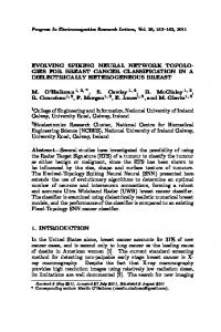
reconfiguration, independent designs (ID) and multi-column partial reconfiguration, communication between designs (CBD). Under the SBM style the designer manually edit low-level changes. Using the FPGA Editor the designer can change the configuration of several components, such as: look-up-table (LUT) equations, internal RAM contents, I/O standards, multiplexers, flip-flop initialization and reset values. However, it is recommended to not change any property or value that could change routing, as it could produce internal contentions and damage the device. After editing the changes, a bitstream containing only the differences between the before and after designs can be generated. For neural-network implementations SBM results inaccurate due to the low- level edition and the lack of automation in the generation of the bitstreams. ID and CBD allow the designer to split the whole system in modules [2]. For each module, the designer must go from the HDL description through the synthesis, mapping, placement, and routing on the FPGA, independently of other modules. Placement and timing constraints are set for each module and for the whole system. Among these modules some are reconfigurable and others fixed (Figure 1). A complete initial bitstream is generated for the fixed along with the initial reconfigurable modules. Partial bitstreams are generated for the reconfigurable modules.
Fig. 1. Design Layout with Two Reconfigurable Modules (figure from [3]).
The difference between these two styles of reconfiguration is that CBD allows the inter-connection of modules through a special bus macro, while ID does not. This bus macro guarantees that, each time partial reconfiguration is performed the routing channels between modules remain unchanged, avoiding contentions inside the FPGA and keeping correct connections between modules. While ID results limited for neural-network implementation, because it does not support communication among modules preventing any connectivity to be done, CBD is well suited for implementing layered topologies of networks where each layer matches with a module. CBD has some placement constraints, among which: (1) the size and the position of a module cannot be changed, (2) input-output blocks (IOBs) are exclusively accessible by contiguous modules, (3) reconfigurable modules can communicate only with
neighbor modules, and it must be done through bus macros (See Figure 1), and (4) no global signals are allowed (e.g., global reset), with the exception of clocks that use a different bitstream and routing channels (more details on [3]).
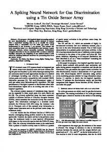
3. Neural Models The inherent parallelism of neural network models has led to the design of a large variety of hardware implementations. Applications as image processing, speech synthesis and analysis, high energy physics, and so on, have found in neural hardware a field with promising solutions. When implemented on hardware, neural networks can take full advantage of their inherent parallelism and run orders of magnitude faster than software simulations, becoming thus, adequate for real-time applications. Most neuron models use continuous values as inputs and outputs, processed using logistic, gaussian or other continuous functions [4,7]. In contrast, biological neurons process pulses: as a neuron receives input pulses by its dendrites, its membrane potential increases according to a post-synaptic response. When the membrane potential reaches a certain threshold value, the neuron fires, and generates an output pulse through the axon. The best known biological model is the Hodgkin and Huxley model (H&H) [9], which is based on the ion current activities through the neuron membrane. However, the most biologically plausible models are not well suited for computational implementations. This is the reason why other different approaches are needed. The leaky integrate and fire (LI&F) model [1,10] is based on a current integrator, modeled as a resistance and a capacitor in parallel. Differential equations describe the voltage given by the capacitor charge, and when a certain voltage is reached the neuron fires. The spike response model order 0 (SRM0) [1,10] offers a similar response to that of the LI&F model, with the difference that, in this case, the membrane potential is expressed in terms of kernel functions instead of differential equations. Spiking-neuron models process discrete values representing the presence or absence of spikes; this fact allows a simple connectionism structure at the network level and a striking simplicity at the neuron level. However, implementing models like SRM0 and LI&F on digital hardware is largely inefficient, wasting many hardware resources and exhibiting a large latency due to the implementation of kernels and numeric integrations. This is why a functional hardware-oriented model is necessary to achieve fast architectures at a reasonable chip area cost. 3.1. The proposed neuron model So as to exploit the coding capabilities of spiking neurons, our simplified model [12], as standard spiking models, uses the following five concepts: (1) membrane potential, (2) resting potential, (3) threshold potential, (4) postsynaptic response, and (5) afterspike response (see figure 2). A spike is represented by a pulse. The model is implemented as a Moore finite state machine. Two states, operational and refractory, are allowed (see figure 2).
Figure 2. Response of the model to a train of input spikes.
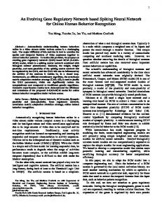
During the operational state the membrane potential is increased (or decreased) each time a pulse is received by an excitatory (or inhibitory) synapse, and then it decreases (or increases) with a constant slope until the arrival to the resting value. If a pulse arrives when a previous postsynaptic potential is still active, its action is added to the previous one. When a firing condition is fulfilled (i.e., potential ≥ threshold) the neuron fires, the potential takes on a hyperpolarization value called after-spike potential and the neuron passes then to the refractory state. After firing, the neuron enters in a refractory period in which it recovers from the after-spike potential to the resting potential. Two kinds of refractoriness are allowed: absolute and partial. Under absolute refractoriness, input spikes are ignored. Under partial refractoriness, the effect of input spikes is attenuated by a constant factor. The refractory state acts like a timer that determines the time needed by a neuron to recover from a firing; the time is completed when the membrane potential reaches the resting potential, and the neuron comes back to the operational state. Our model simplifies some features with respect to SRM0 and LI&F, specifically: the post-synaptic and the after-spike responses. The way in which several input spikes are processed affects the dynamics of the system: under the presence of 2 simultaneous input spikes, SRM0 performs an addition of post-synaptic responses, while our model adds the synaptic weights to the membrane potential. Even though our model is less biologically plausible than SRM0 and LI&F, it is still functionally adequate. 3.2 The proposed neuron on hardware The hardware implementation of our neuron model is illustrated in Figure 3. The computing of a time slice (iteration) is given by a pulse at the input clk_div, and takes a certain number of clock cycles depending on the number of inputs to the neuron. The synaptic weights are stored on a memory, which is swept by a counter. Under the presence of an input spike, its respective weight is enabled to be added to the membrane potential. Likely, the decreasing and increasing slopes (for the post-synaptic and after-spike responses respectively) have been previously stored on the memory.
Figure 3. (a) External view of the neuron. (b) Architecture of a neuron.
Although the number of inputs to the neuron is parameterizable, increasing the number of inputs implies raising both: the area cost and the latency of the system. Indeed, the area cost highly depends on the memory size, which itself depends on the number of inputs to the neuron (e.g. the 16x9-neuron on figure 3 has a memory size of 16x9 bits, where the 16 positions correspond to up to 14 input weights and the predefined increasing and decreasing slopes; 9 bits is the arbitrarily chosen data-bus size). The time required to compute a time slice is equivalent to, at least, the number of inputs +1 (up to 14 inputs plus either the increasing or the decreasing slope). We have also designed two other larger neurons: a 32x9 and a 64x9-neuron. Each one of them requires a larger memory and larger combinatorial logic to manage the inputs. Some synthesis results from the implementation of these neurons on a Virtex II-pro vc2vp4 FPGA are illustrated on Table 1. The area requirement is very low compared to other more biologically-plausible implementations (e.g. Ros et al [6] use 7331 Virtex-E CLB slices for 2 neurons). Table 1. Resource requirements for a single neuron on a Virtex II-pro vc2vp4.
16x9-neuron (14 inputs) 32x9-neuron (30 inputs) 64x9-neuron (62 inputs)
17 CLB slices 33 function generators 23 CLB slices 45 function generators 46 CLB slices 92 function generators
0.57% 0.55% 0.75% 0.76% 1.53% 1.53%
4. On-line Evolution Three main types of neural network evolutionary approaches might be identified: evolution of synaptic weights, evolution of learning rules, and evolution of topologies [11]. Evolution of synaptic weights (learning by evolution) is far more time-
consuming than other learning algorithms. Evolution of learning rules, where we search for an optimal learning rule, could be of further interest for our methodology. Evolution of topologies is the most interesting as it allows the exploration of a wider search space and, combined with weight learning, is a very powerful problem solver. The main consequence of the features of DPR is a modular structure, where each module communicate solely with his neighbor modules through a bus macro (Figure 1). This structure matches well with a layered neural-network topology, where each reconfigurable module contains a layer. Inputs and outputs of the full network should be previously fixed, as well as the number of layers and the connectivity among them (number and direction of connections). While each layer can have whatever kind of internal connectivity, connections among them are restricted to neighbor layers. For each module, there exists a pool of different possible configurations. A simple genetic algorithm [5] is the responsible for determining which configuration is going to be active. As illustrated in figure 4, each module can be configured with several different layer topologies, provided that they offer the same external view (i.e. the same inputs and outputs).
Figure 4. Layout of the reconfigurable network topology
The genetic algorithm considers a full network as an individual. Several generic layer configurations are generated to obtain a library of layers, which can be used for different applications; however, for each application the genetic algorithm finds the combination of them that best solves the problem. Fixed modules contain the required logic to code and decode inputs and outputs and to evaluate the fitness of the individual depending on the application (the fitness could also be evaluated on the PC). Given n modules, corresponding to an n-layer neural-network and c(i) possible configurations for the i-th module (i = 1,2,…n), the genome contains n genes, each gene determining which configuration is downloaded to each module. The binary encoding length of the i-th gene is l(i) = log2(c(i)). The full genome-length is given by L=∑l(i).
5. Conclusions and future work In this paper we present a methodology to evolve hardware neural networks on-line. Although our methodology has been conceived for spiking neural-networks, it is
applicable to any kind of digital neural hardware. Our long-term goal is to develop a tool including a library of generic neural layers, which allow the user to select the desired type of neuron, the number of layers, number of neurons-per-layer and the connectivity among them. Spiking-neuron models seem to be the best choice for this kind of implementation, given their low requirements of hardware and connectivity, keeping good computational capabilities, compared to other neuron models [10]. Likewise, layered network topology, which is one of the most commonly used, seems to be the most suitable for our implementation method. However, other topologies are still to be explored. Different space search techniques could be applied with our methodology. Genetic algorithms constitute one of the most generic, simple, and well known of these techniques but we are convinced that it is not the best one. It does not take into account information that could be useful to optimize the network, such as the direction of the error. An example of this could be found on [4] where growing and pruning techniques are used to find the correct size of a network. In a more general way, this work could be considered for any hardware structure with adaptivity requirements. For example fuzzy systems could be evolved in a structural way, finding the best fuzzification, inference, rules, and defuzzification stages, considering each one of them as a layer of the system, and creating libraries of parameterizable modules. On the same way it applies to processor architectures, signal processing, cellular automata, statistical methods, etc.
References 1. W. Gerstner, Kistler W. Spiking neuron models. Cambridge University Press. 2002. 2. Development System Reference Guide. Xilinx corp. www.xilinx.com. 3. D. Lim, M. Peattie. XAPP 290: Two Flows for Partial Reconfiguration: Module Based or Small Bits Manipulations. May 17, 2002. www.xilinx.com 4. A. Perez-Uribe. Structure-adaptable digital neural networks. PhD thesis. 1999. EPFL. http://lslwww.epfl.ch/pages/publications/rcnt_theses/perez/PerezU_thesis.pdf 5. M. Vose. The Simple Genetic Algorithm: Foundations and Theory. MIT Press, 1999. 6. E. Ros, R. Agis, R. R. Carrillo E. M. Ortigosa. Post-synaptic Time-Dependent Conductances in Spiking Neurons: FPGA Implementation of a Flexible Cell Model. Proceedings of IWANN'03: LNCS 2687, pp 145-152, Springer, Berlin, 2003. 7. S. Haykin. Neural Networks, A Comprehensive Foundation. 2 ed, Prentice-Hall, Inc, New Jersey, 1999. 8. R. Reed, Pruning Algorithms – A Survey. IEEE Transactions on Neural Networks 1993; 4(5):740-747. 9. A. L. Hodgkin, and A. F. Huxley, (1952). A quantitative description of ion currents and its applications to conduction and excitation in nerve membranes. J. Physiol. (Lond.), 117:500544 10. W. Maass, Ch. Bishop. Pulsed Neural Networks. The MIT Press, Massachusetts, 1999. 11. X. Yao. Evolving artificial neural networks. Proceedings of the IEEE, 87(9):1423-1447, September 1999. 12. A. Upegui, C.A. Peña-Reyes, E. Sánchez. A Functional Spiking Neuron Hardware Oriented Model. Proceedings of IWANN'03: LNCS 2686, pp 136-143, Springer, Berlin, 2003.