Evolving Spiking Neural Network Controllers for. Autonomous Robots. Hani Hagras, Anthony Pounds-Cornish, Martin Colley, Victor Callaghan and Graham ...
Evolving Spiking Neural Network Controllers for Autonomous Robots Hani Hagras, Anthony Pounds-Cornish, Martin Colley, Victor Callaghan and Graham Clarke Department of Computer Science University of Essex Wivenhoe Park, Colchester, CO4 3SQ, UK Email: {hani, apound, martin, vic, graham}@essex.ac.uk Abstract— In this paper we introduce a novel mechanism for controlling autonomous mobile robots that is based on using Spiking Neural Networks (SNNs). SNNs are inspired by biological neurons that communicate using pulses or spikes. As SNNs have shown to be excellent control systems for biological organisms, they have the potential to produce good control systems for autonomous robots. In this paper we present the use and benefits of SNNs for mobile robot control. We also present an adaptive Genetic Algorithm (GA) to evolve the weights of the SNNs online using real robots. The adaptive GA using adaptive crossover and mutation converge in a small number of generations to solutions that allow the robots to complete the desired tasks. We have performed many experiments using real mobile robots to test the evolved SNNs in which the SNNs provided a good response. Index terms - spiking neural network; genetic algorithms; autonmous mobile robots; robot navigation; fuzzy controllers
I.
INTRODUCTION
This work is part of a European Union funded project entitled “Self-Organised Societies of Connectionist intelligent Agents capable of Learning" (No IST-2001-38911). The three year project’s aim is to produce nano-scale autonomous robots capable of achieving well defined tasks in difficult, challenging and inaccessible environments. An application benchmark for this project is the on-line maintenance and repair of filters for organ replacement therapy systems. Most biological neurons communicate by sending pulses across connections to other neurons [1]. The pulse is also known as a “spike” to indicate its short and transient nature [2]. Such neurons are called spiking neurons and their networks are termed Spiking Neural Networks (SNNs). As biological organisms have shown to be excellent control systems using SNNs then SNNs have the potential to produce good control systems for autonomous robots [2]. SNNs are deemed computationally more powerful than conventional artificial neural network formalisms on the basis of extensive theoretical work by Maass [3]. “Computationally more powerful” implies that SNNs need fewer nodes to solve the same problem than conventional artificial neural networks [3]. From an implementation viewpoint, this means that SNN circuits of the same complexity can provide “more for less”
compared to other neural network implementations (such as the multi layer perceptrons). In addition, SNNs provide a number of other desirable features such as noise-robustness (tolerance to background noise) and simple real-world interfaces [4]. The computational power of SNNs exist because of the intrinsic time-dependent dynamics of spiking neurons that allow the temporal patterns of sensory-motor events to be captured and exploited more efficiently than the other connectionist models (i.e. with fewer neurons and simpler circuits) [1,3]. Moreover, SNNs can be mapped easily to hardware because the spikes are in essence binary events and the non linear dynamics and the coding of spiking circuits can be provided by spiking times, rather than by non linear, real valued activation functions used in the traditional connectionist neuron models [2]. In other words, a few logic operations and instructions to move around single bits over time would be sufficient to embed large circuits of spiking neurons that display complex abilities and behaviours into tiny and low power chips. Therefore such SNNs will be appropriate control mechanisms for our nano-scale autonomous robots as they can give a very good response dealing with noise using tiny chips that consume little power in inaccessible environments. This is a big advantage especially as both memory and power are extremely limited on the micro and nano-scale platforms currently being developed by the project. There have been many applications of SNNs to robotics; most of these applications are focused on the first stages of sensory processing and on relatively simple motor control. For example [5] developed neuromorphic vision circuits that emulate interconnections among neurons in the early layers of the biological retina in order to extract motion information and implement a simple form of attentive selection. These vision circuits have been interfaced with a robot to follow lines. In [6] they developed an analog VLSI circuit with four spiking neurons capable of controlling a robotic leg and adapting the motor commands using sensory feedback. This circuit’s size is less than 0.4 mm2 and it consumes less than 1 microwatt. Despite these interesting implementations, they did not produce methods for developing complex SNNs that could display minimally cognitive functions or learn their behaviours through autonomous interactions with their environment [1]. Implementations of SNNs are difficult as the hand design of
SNNs that display a desired functionality is not a trivial task because of the highly non linear dynamics [2]. Furthermore, the learning algorithms developed for SNNs are often restricted to very simple and application specific architectures [7]. Artificial evolution through Genetic Algorithms (GAs) is therefore an interesting method to discover SNNs that autonomously develop desired behaviours for robots without imposing constraints on their architecture and functioning modality. GAs have been used to evolve SNNs for a task of vision-based navigation using a Khepera robot to navigate in a rectangular arena with textured walls [1]. Implementation of these SNNs in digital microcontrollers with size and power consumption competitive with analog VLSI chips has also been described [2]. Their controller was implemented in a small robot only 2 cm long [2]. However in [1,2] they evolved only the signs of the SNN’ s weights leaving the values of weights constant to 1. They have used a GA with fixed crossover and mutation probabilities and they have used a large population of 60 chromosomes. Their GA converged after 30 generations where each generation took about 80 minutes using the real robots, so their GA converged after approximately 40 hours. In this paper we introduce an adaptive GA which uses adaptive crossover and mutation probabilities. We used our adaptive GA to evolve the weight values and signs of the SNNs online in a relatively short time interval using real robots interacting with their environment. We will show many experiments in which we evolved good SNN controllers in a small number of generations. In Section II we will introduce SNNs and their operation. Section III introduces the online adaptive GA. The application of SNNs to mobile robots is introduced in Section IV. Experimental results are introduced in Section V and conclusions and future work are presented in Section VI. II.
SPIKING NEURAL NETWORKS
The “ time aspect” of SNNs is responsible for their computational power. In virtually every artificial computing machine one is keen to ensure that the timing of individual computation steps adheres to a global schedule, which is independent of the values of the input variables [3]. For example, layer d of a feed forward neural network is required to produce its output at step Kd of the computation regardless of the values of the inputs to the network [3]. In contrast to that, the firing times of neurons in a biological neural system depend on the input to that system [3]. Hence networks of spiking neurons (which are very close to the real world biological neural network) are capable of exploiting time as a resource for coding and computation in a much more sophisticated manner than virtually all other common computational models [7,8]. The state of a spiking neuron is described by the voltage difference across its membrane, also known as membrane potential v [1]. Incoming spikes can increase or decrease the membrane potential. The neuron emits a spike when the total amount of excitation induced by the incoming excitatory and inhibitory spikes exceeds its firing threshold . After firing, the membrane potential of the neuron resets its state to a low negative voltage during which it cannot emit a new spike, and
it gradually returns to its resting potential. The recharging period is called the refractory period. There are several models of spiking neurons that account for these properties with various degrees of detail. In this paper we will use the Spike Response Model (SRM) [9]. It has been shown that several other models of spiking neurons, such as the class of Integrate and Fire neurons (where the membrane potential of the neuron is immediately reset to its resting value after a spike), represent special cases of the Spike Response Model [1,9]. In the SRM, the effect ε of an incoming spike on the neuron membrane is a function of the difference
s = t −t f .
(1)
Where t is the current time and t f is the time when the spike was emitted (firing time). The properties of the function are determined by the following: •
The delay ∆ between the generation of a spike at the pre-synaptic neuron and the time of arrival at the synapse.
•
A synaptic time constant τs.
•
A membrane time constant τm.
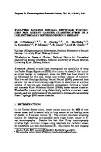
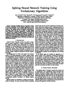
The idea is that a spike emitted by a pre-synaptic neuron takes some time to travel along the axon and once it has reached the synapse, its contribution to the membrane potential is higher as soon as it arrives but gradually fades as time passes [1]. A possible function ε(s) describing this behaviour is shown in Fig. 1(a) and can be written as follows [1]:
ε (s ) = exp[− (s − ∆ ) τ m ](1 − exp[− (s − ∆ ) τ s ]): s ≥ ∆ 0 : s < ∆ . (2) Once a neuron has emitted a spike, its membrane potential is set to a very low value to prevent an immediate second spike and then it gradually recovers to its resting potential. The speed of recovery depends on the membrane time constant τm. A possible function η(s), for this refractory period is shown in Fig. 1(b) and can be written as follows [1,9]
η (s ) = − exp[− s τ m ].
(3)
We can now put together the equations describing synaptic contributions and the refractory period to describe the dynamics of a neuron that has several synaptic connections from the input neurons. Each synaptic connection has a weight wij which can be negative (inhibitory) or positive (excitatory). The membrane potential of a neuron i at time tc is given by tc
vi (t c ) = ∑ j =1 wij ∑tc=1 ε j ( s j ) + ∑η i ( si ) . N
t
(4)
t =1
Where j is the pre-synaptic neuron and i is the post-synaptic neuron. wij is the weight of the synaptic connection between neuron i and neuron j. N is the total number of the pre-synaptic neurons. tc is the current time. sj is an application of (1) for the
pre-synaptic neuron j and si is an application of (1) for the postsynaptic neuron i.
t jf = T − kx j .
(5)
Where T is the time of the control cycle (100 ms in our case) and k is a suitable scaling factor.
Figure 1. (a) Function describing ε (b) Function describing refractory period
If the membrane potential vi(tc) is equal to or larger than the neuron threshold θi, the neuron emits a spike (fires) at tif and ηi takes a very low value that prevents an immediate new spike. After that, ηi is computed according to (3). As it is complex to solve (4) [10], in each control cycle which takes T time steps we will iterate over tc to find when (4) exceeds the threshold at the time the spike was emitted. For our robots the control cycle takes 100 ms thus we have set T to be 100 and each time step is 1 ms. In our SNNs the robot sensor inputs are connected to the pre-synaptic neurons, while the actuator’ s outputs are connected to the post-synaptic neurons. In SNNs, a single spike is a binary event that can encode only the presence or absence of a stimulus. There are many ways of mapping the sensor’ s analog value to spikes at the beginning of the control cycle. One method consists of mapping the sensor analog value to the firing rate of the neuron; this method is based on the hypothesis that a neuron increases its firing rate to indicate a high analog sensor value [1]. This is biologically inspired from the frog in which the firing rate of a stretch receptor in the frog’ s leg is a monotonically increasing function of the strength of stimulation [11]. Another method for mapping consists of encoding the sensory stimulation across several neurons and mapping the intensity of the stimulation into the number of neurons that spike at the same time [1]. This method is based on the hypothesis that the brain represents meaningful information by synchronising spiking activities across several neurons, this has been supported by measurements in the visual and temporal cortex of monkeys [12]. Another method for mapping sensor values to spikes consists of encoding the strength of the sensor value in the firing delay of the neuron. The underlying hypothesis is that neurons that receive stronger stimulation fire earlier than neurons receiving weaker stimulation, so highly stimulated neurons tend to spike sooner. This has been supported by measurements in olfactory neurons [13]. In this paper, we use the latter method for mapping sensor analog values to spikes. This coding system known as “ delay coding” or “ latency coding” has been used by many researchers as it is simple and it is one of very few coding methods that might theoretically be used for very fast neural computation [8,14,15] which is required in our problem domain. For an analog input sensor value xj to pre-synaptic neuron j, the firing time tjf can be calculated as follows [14]
At the end of the control cycle, we need to convert the firing of the post-synaptic neuron i, to analog outputs for the actuators. We are going to use the delay coding again, so the analog output yi passed to the actuator connected to neuron i can be written as follows:
yi =
T − ti f . c
(6)
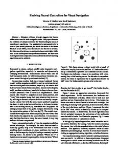
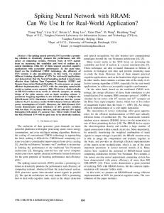
Where c is a suitable scaling factor, tif is the firing time for the post-synaptic neuron i. The generic architecture of an SRM SNN using delay coding is shown in Fig. 2. III.
ONLINE GENETIC ALGORITHMS
Adaptive behaviours in robots cannot be considered as a product of the robot in isolation from the world, but can only emerge from a strong coupling of the robot and its environment [16]. It is desirable that the robots learn their own behaviour online through interacting with their real environment rather than relying totally on simulations. The fact that it is very hard to simulate the actual dynamics of the real world implies that effort will go into solving problems that exist only in the simulation. Additionally, programs which work well on simulated robots might not work properly on real robots [17]. Not only are implementations of SNNs difficult to hand craft [2] but the learning algorithms developed for SNNs are often restricted to very simple and application specific architectures [7]. For the mobile robot domain there is a need to produce methods for developing complex SNNs that could display minimally cognitive functions and learn their behaviours through autonomous interactions with the environment [1]. ANALOG SENSORS
INPUT SPIKES
INPUT UNITS
OUTPUT UNITS
OUTPUT SPIKES
ANALOG OUTPUT
t
s1
x1
i1
f 1
t
w11
t2f
y1
t1f
w12
s2 x2
o1
i2
o2
t 2f
y2
w1i sj xj
ij
t jf
T
wji
oi
ti f
yi
Figure 2. SRM SNN using delay coding architecture
Artificial evolution through Genetic Algorithms (GAs) is therefore a useful method to discover SNNs that autonomously develop behaviours for robots without imposing constraints on their architecture and functioning modality. GAs are a biologically inspired class of algorithms which do not rely on
any analytical properties of the function to be optimised (such as an existence of a derivative). They are capable of performing an intelligent search for a solution from a nearly infinitely sized problem space [18]. GAs are suited to a wide class of problems and they are particularly suitable for solving complex optimisation problems and therefore suitable for applications that require adaptive problem-solving strategies [18]. Standard GAs are widely known to be slow as they usually require big populations and they only converge after a large number of generations. This limits their application to mobile robot online learning [18]. However we can use adaptive online GAs, rather than standard GAs to find good enough solutions in a relatively short time interval [18]. Using online GAs, it is desirable to achieve a high level of online performance whilst being capable of reacting rapidly to changes requiring new actions [18]. Hence it is necessary to maintain a limited amount of exploration and diversity in the population. These requirements mean that the population size should be kept sufficiently small, so that progression towards near-convergence can be achieved within a relatively short time [18]. Similarly the genetic operators (crossover and mutation) should be used in a way that rapidly achieves high-fitness individuals in the population [18]. In our online GAs we will use small population sizes and we are going to use adaptive genetic parameters to speed up the search process. We will use a novel method to adaptively change the crossover and mutation probabilities based on Srinivas method [19]. This method helps us to achieve good crossover and mutation parameters that aid convergence in a short time interval. The strategy used for adapting the control parameters depends on the definition of the performance of the GA. The GA should possess the capacity to track optimal solutions and the adaptation strategy needs to vary the control parameters appropriately whenever the GA is not able to track the located optimum [19]. There are two essential characteristics that must exist in the GA for optimisation. The first characteristic is the capacity to converge to an optimum (local or global) after locating the region containing the optimum [19]. The second characteristic is the capacity to explore new regions of the solution space in search of the global optimum [19]. In order to vary Pc (crossover probability) and Pm (mutation probability) adaptively to prevent premature convergence of the GA, it is essential to be able to identify whether the GA is converging to an optimum. One possible way of detecting convergence is to observe the average fitness value f of the population in relation to the maximum fitness value fmax of the population. fmax - f is likely to be less for a population that has converged to an optimum solution than that for a population scattered in the solution space. Pc and Pm are defined as follows:
f max - f ′′ : f ′′ ≥ f ′ f max − f ′ Pc = 1 : f ′′ < f ′ f max − f Pm = : f ≥ f′ 2( f max − f ’) Pm = 0.5 : f < f ′ Pc =
(7)
(8)
Where f is the larger of the fitness values of the solutions to be crossed. f is the fitness of the individual solutions. The method means that we have Pc and Pm for each chromosome. The type of crossover was chosen to be a one point crossover for computational simplicity and real time performance. One of the goals of this approach is to prevent the GA from getting stuck in a local optimum. As we are using small population sizes, we employ a high Pm value of 0.5 to the average and sub average fitness chromosomes to introduce new genetic material without reducing the search process to a random process [19]. The same for the Pc which takes a value of 1.0 to ensure that average and sub average fitness chromosomes undergo crossover. In [19] they proved that this method was superior to the simple GA and gave a faster convergence rate of 8:1. This approach produces fast converging solutions and adapts the GA for non-static environments [16]. It also relieves the designer from determining these values heuristically [16]. IV.
APPLICATION OF SNNS TO MOBILE ROBOT CONTROL
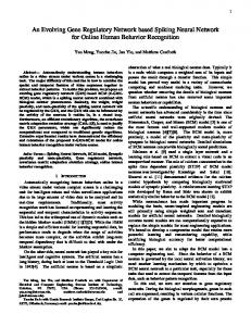
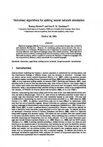
We are going to apply our SNNs to the control of the mobile robot shown in Fig. 3(a). The robot features two independently controllable wheels and a bank of nine ultrasound sensors. These ultrasound sensors are made up of an emitter and receiver pair as shown in Fig. 3(b). All of the ultrasound sensors are time multiplexed such that they do not interfere with each other. The wheels are connected to stepper motors which are capable of variable speeds, both forwards and in reverse. The robot is also equipped with four overlapping bump sensors which enable the robot to know when it has collided with an obstacle.
Figure 3. (a) The robot (b) One of the ultrasound sensors used
The robot runs the VxWorks operating system and is programmed by compiling C code with the appropriate robot libraries into an object file which can be loaded into the robot’ s memory for execution. Communication with the robot is achieved across Wireless LAN 802.11b using both the Telnet and File Transfer (FTP) protocols. The robot also includes a rechargeable battery that allows it to run wirelessly for approximately 2.5 hours. We have used ultrasound sensors as they represent the sort of sensors to be used in our nano robots. The ultrasound
sensors used are noisy and imprecise so they allow us to evaluate the performance of the SNNs under these conditions. In our SNNs, we use a two layer structure, in which the ultrasound sensors’ analog value will be the inputs to the SNN’ s pre-synaptic neurons and the analog values from the post-synaptic neurons will be the outputs to the actuators. So in the case of the right edge following behaviour, using the two right side sensors means we will have two pre-synaptic neurons. As we have two actuators which are the left and right motor speeds, we have two post-synaptic neurons and thus we will have four weights connecting the two pre-synaptic neurons to the two post-synaptic neurons. To evolve the SNN controller online we evolve the values and signs of the weights of the SNNs; the weights take any value between -1 and +1 and we use binary coding in our online GAs. The chromosome which represents a possible solution for the problem consists of all the weights in the SNN and we represent each weight by 5 binary bits. The bit strings are combinations of 0 and 1s, which represent positive and negative values of the weights in a binary form. An n-bit string can accommodate all integers up to the value 2n – 1. So using 5 bits can represent 25 = 32 integer values, where a weight of +1 will be equivalent to an integer value of 31, a weight of -1 will be equivalent to an integer value of 0 and a weight of 0 (i.e. no connection) will be equivalent to an integer value of 15. Consequently positive weight values between 0 and +1 will be equivalent to integer values between 15 and 31 and the negative weight values between -1 and 0 will be equivalent to integer values between 0 and 15. In this way we can evolve the signs and values of the weights of the SNN. When testing a chromosome the weight binary value is mapped back into a real weight value between -1 and +1 and applied to the SNN controller which the robot uses to move. In the case of the right edge following behaviour, each chromosome will code four weights and each weight will be coded by 5 bits, therefore each chromosome will consist of 5*4 = 20 bits. As we are using online GAs we have to use small population sizes; we have used a population of 4 chromosomes in our experiments. In all our experiments the robot is started from a random location with a random chromosome (i.e. random weights). The robot then moves forward a constant distance to test each chromosome solution. At the end of this testing, each chromosome is allocated a level of fitness according to how well it did the specified job. This is repeated until each chromosome in the population has been evaluated and assigned a level of fitness. We then use the adaptive crossover and mutation explained in Section III to generate a new population of chromosomes. We used an elite strategy, meaning that the best individual is automatically promoted to the next generation and used to generate subsequent populations. The search for the solution stops when the stopping criterion of achieving the desired performance is met. In the next section we will show many experiments evolving the SNN controllers for mobile robots.
V.
EXPERIMENTS AND RESULTS
We have performed many experiments to evaluate the performance of the SNN controller in mobile robots. Due to the limited space we will only introduce as a proof of concept experiments related to evolving the right edge following behaviour which is needed by the nano robots in our project. The aim of the right edge following behaviour is to follow the edge at a desired distance. As we explained above we used the front and back right side sensors as inputs to two pre-synaptic neurons and the two post-synaptic neuron outputs were fed to the left and right motor speeds. We used the online GAs to optimise the values and signs of the weights as well as their existence, for example if weight w11 is optimised by the GAs to be zero, then w11 can be removed from the SNN to optimise its architecture. The fitness of each solution (Chromosome) proposed by the GA can be written as 1 – the scaled average deviation from the desired distance. Thus the GA maximises its fitness by minimising the average deviation from following the edge at the desired distance. The robot path was drawn using a pen fixed to the back of the robot. In the following experiments we used noisy ultrasound sensors and different irregular geometrical structures which cause multiple reflections and sonar diffuse reflection. We used these noisy sensors and environments in order to test the ability of SNNs to deal with noisy environments. In all the following experiments, all the scaled average and standard deviations from the desired values were calculated over four experiments, where we used different geometrical structures, started the robot from different random locations and used different desired wall following distances for the right edge following behaviour. The deviations are scaled to have values between 0 and 1. To test the quality of the evolved solutions we started experiments using handcrafted SNNs in which all the weights were either +1, 0 or -1 as used by [1,2]. The SNN controller has given a good response as shown in Fig. 4. The robot had given a scaled average deviation of 0.23 and an absolute standard deviation of 0.16.
Figure 4. The handcrafted SNN path
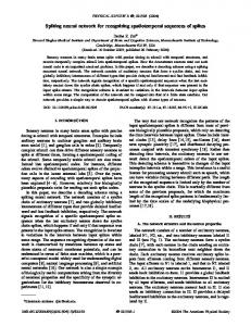
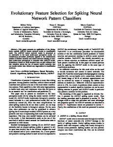
We then performed more experiments to compare the SNNs evolved using the adaptive online GA to the SNNs evolved using a standard GA to show the benefits of the former. The standard GA used the same population size as the adaptive online GA and it used fixed crossover and mutation probabilities. Fig. 5 shows the results from the comparison
between the standard GA and the online GA using adaptive crossover and mutation probabilities. Adaptive GA
Static GA
0.9
These experiments have shown that the SNNs which provide a fast processing system, provide very good performance in the face of noise and imprecision.
0.89 WALL FOLLOWING FITNESS
shown in Fig. 6, the SNN controller provides a much smoother response when compared to the FLC, whilst the FLC has a worse scaled average deviation. Also in all cases the SNN controller response was repeatable in face of noise, but the FLC failed in some cases and collided with the walls.
0.88 0.87 0.86 0.85 0.84 0.83 1
2
3
4
5
6
7
8
9
10
11
12
13
14
15
NUMBER OF GENERATIONS PASSED
Figure 5. Average GA fitness agianst number of generations
Fig. 5 shows the average fitness of the population (over four experiments) plotted against each generation in the GA cycle. The dotted line represents the progress of the standard GA’ s attempt to improve the quality of the wall following SNN. The solid line represents the progress of the adaptive online GA. It can be seen that both the standard and the adaptive online GA provide a large initial improvement in the average fitness of the solutions in the 1st to 3rd generation which outperform the hand crafted SNN. In the first few generations the indicative benefit of using GAs to evolve the SNNs weights can be seen. However the standard GA and the adaptive GA both suffer from the local minima problem as can be seen in the flat part of both lines from generations 3 to 9. The adaptive GA using the adaptive mutation and crossover probabilities can escape from the local minima and satisfy the desired stopping criteria giving a very good best scaled average deviation of 0.0973 whilst the standard GA was stuck in an area of local minima and could not achieve the desired stopping criteria. The adaptive online GA had converged to the required solution and satisfied the stopping criteria after only 14 generations which took 40 minutes of the robot’ s time where most of the time was consumed in moving the robot forward and backward to its starting position to test a new chromosome. So using our online GAs which use small population sizes and adaptive crossover and mutation probabilities had resulted in converging to the desired solution in a relatively short time interval using the real robots. The values for the evolved SNN weights using our online adaptive GAs are as follows, w11 = 0.453125, w12 = -0.25, w21 = 0.468750, w22 = -0.25. The evolved SNN has shown to have a very good response in the face of noise, uncertainty and imprecision as shown in Fig. 6, where it gave a best scaled average deviation of 0.0973 starting the robot from different starting positions and using different obstacles and geometrical set-ups. We have also compared the SNN controller against a well known technique for dealing with noise, uncertainty and imprecision which is the Fuzzy Logic Controller (FLC). As
Figure 6. Wall following path of SNN and Fuzzy controllers
VI.
CONCLUSIONS AND FUTURE WORK
In this paper, we have introduced a novel controller for a mobile robot that is based on SNNs. SNNs are inspired from biological neural networks and they provide a fast processing system that provide tolerance to background noise. They can also be mapped in small programs and thus requires few logic operations and instructions to move around single bits. Thus large SNNs can be embedded in tiny and low power chips that can achieve complex tasks and behaviours. Such SNNs will be appropriate control mechanisms for the nano-scale autonomous robots developed by our project as they can give a very good response when dealing with noisy, inaccessible environments whilst consuming little power. This is a big advantage especially considering that both memory and power are extremely limited on the micro and nano-scale platforms currently being developed by the project. We have presented an adaptive online GA based system that was used to evolve the SNN controller online through interaction with the real environment; it converged in a relatively short time interval in a small number of generations and produced a very good solution that outperformed the standard GA. The evolved SNN controller also provided an acceptable solution to the wall following problem even when compared with a Fuzzy controller benchmark; the SNN controller gave a smoother and better response. The results shown in this paper for the edge following behaviours only provide sample behaviour as we have also developed other SNN behaviours. Also, we are currently working on evolving more complex behaviour that is needed by nano robots in three dimensional environments. As part of the project we are currently mapping the evolved SNN controller to evolvable FPGA hardware.
Much of the time in GA evolution was spent waiting for robot to return to the starting position. It has been a popular trait in mobile robot research to use simulation rather than real robots to produce solutions. However, previous experience has shown that solutions evolved in a simulated environment rarely function as well or even as expected when placed back into the real world. With this in mind, we are currently working on a simulator for the robot that is able to work alongside real world experiments. For our future work we intend to extend the online GAs to evolve other parameters of the SNNs like the membrane and synaptic time constant. The ultimate goal in this thread of research is to produce an adaptive GA that is able to evolve both the parameters and the structure of the SNN to produce solutions to more complex behavioural problems.
[4] [5] [6]
[7] [8] [9] [10]
By the end of the project we hope to implement SNNs on VLSI to produce controllers for small robots. These small robots will communicate with each other to collaboratively solve problems in complex and inaccessible environments.
[12]
ACKNOWLEDGMENT
[13]
We are pleased to acknowledge the funding support from the EU Future and Emerging Technology programme for the project entitled "Self-Organised Societies of Connectionist Intelligent Agents capable of Learning ", No IST-2001-38911. We are also pleased to acknowledge our project partners: the University of Patras, Greece; CTI, Greece and NMRC, Ireland. REFERENCES [1] [2] [3]
D.Floreano and C.Mattiussi, "Evolution of spiking neural controllers for autonomous vision-based robots," Proceedings of the International Symposium on Evolutionary Robotics (ER-2001), 2001. D.Floreano, N.Schoeni, G.Caprari and J.Blynel, "Evolutionary bits ’n’ spikes," Proceedings of the Eighth International Conference on Artificial Life, 2002. W.Maass, "Networks of spiking neurons: the third generation of neural network models," Australian Conference on Neural Networks, 1996.
[11]
[14] [15] [16] [17] [18] [19]
T.Lehmann and R.Woodburn, "Biologically-inspired on-chip learning in pulsed neural networks," in Analog Integrated Circuits and Signal Processing, 2 ed., vol. 18. 1999, pp. 117-131. G.Indiveri, "Neuromorphic analog VLSI sensor for visual tracking: circuits and application examples," in IEEE Trans.on Circuits and Systems II, 11 ed., vol. 46. 1999, pp. 1337-1347. M.A.Lewis, R.Etienne-Cummings, A.H.Cohen and M.Hartmann, "Toward biomorphic control using custom VLSI CPG chips," in Proceedings of IEEE International Conference on Robotics and Automation, 2000, pp. 494-500. W.Maass and C.M.Bishop, "Pulsed Neural Networks," 1999. W.Maass, "On the computational complexity of networks of spiking neurons," in Advances in Neural Information Processing Systems, 7. 1995, pp. 183-190. W.Gerstner, J.Leo van Hemmen and J.D.Cowan, "What matters in neuronal locking?," in Neural Computation, 8 ed., vol. 8. 1996, pp. 1653-1676. B.Tonkes, "Simulation issues in spiking neural networks," Proceedings on the Eighth Australian Conference on Neural Networks, 1997. W.Singer, "Search for coherence: a basic principle of cortical selforganization," in Concepts in Neuroscience, 1. 1990, pp. 1-26. W.Singer and C.M.Gray, "Visual feature integration and the temporal correlation hypothesis," in Annual Review of Neuroscience, 18. 1995, pp. 555-586. J.J.Hopfield, "Pattern recognition computation using action potential timing for stimulus representation," 2002. W.Maass, "On the relevance of time in neural computation and learning," in Theoretical Computer Science, 1 ed., vol. 261. 2001, pp. 157-178. S.Thorpe and J.Gautrais, "Rapid visual processing using spike asynchrony," 1997. H.Hagras, V.Callaghan and M.Colley, "Prototyping design and learning in outdoor mobile robots operating in unstructured outdoor environments," 2001. R.A.Brooks, "Artificial Life and Real Robots," Toward a Practice of Autonomous Systems: Proceedings of the First European Conference on Artificial Life, 1992. G.Linkens and O.Nyongeso, "Genetic algorithms for fuzzy control, part II: online system development and application," IEE Proceedings Control Theory Applications, 1995. M.Srinivas and L.Patnaik, Adaptation in Genetic Algorithms in Genetic Algorithms For Pattern Recognition. CRC Press, 1996.