then uses a tabu search based approach to place clusters while enhancing both ... One technology that is evolving very rapidly is field programmable gate array ...
A Methodology for Fast FPGA Floorplanning � John M. Emmert and Dinesh Bhatiay Design Automation Laboratory ECECS Department P.O. Box 210030 University of Cincinnati Cincinnati, OH 45221–0030
fjemmert,dineshg @ececs.uc.edu
Abstract Floorplanning is an important problem in FPGA circuit mapping. As FPGA capacity grows, new innovative approaches will be required for efficiently mapping circuits to FPGAs. In this paper we present a macro based floorplanning methodology suitable for mapping large circuits to large, high density FPGAs. Our method uses clustering techniques to combine macros into clusters, and then uses a tabu search based approach to place clusters while enhancing both circuit routability and performance. Our method is capable of handling both hard (fixed size and shape) macros and soft (fixed size and variable shape) macros. We demonstrate our methodology on several macro based circuit designs and compare the execution speed and quality of results with commercially available CAE tools. Our approach shows a dramatic speedup in execution time without any negative impact on quality. Key Words: Floorplanning, Placement, FPGA, Clustering, Tabu Search
1 Introduction Placement and floorplanning are extensively studied topics. However, the importance of placement and floorplanning cannot ever be ignored due to changing design complexities and requirements. One technology that is evolving very rapidly is field programmable gate array (FPGA). Currently, commercially available devices can map up to one million gate equivalent designs[19] (and some of the newly announced products like Altera’s APEX series will map over two million gate equivalent designs[1]). Such complex design densities also demand tools that can efficiently and quickly make use of available gates. Improvements in CAD tools for FPGAs have not kept pace with hardware improvements. The available tools typically require from minutes to hours to map1 designs (or circuits) with just a few thousand gates, and as design sizes increase the execution time will increase. One way to address the problem of long mapping times is � this work is partially supported by Air Force Research Laboratory of the US Air Force under contract number F33615-97-C-1043 ycorresponding author 1 typical mapping steps include technology mapping, placement, and routing
create designs that use premapped macros2 to create larger designs (macro based circuits). Then we floorplan and route these macro based circuits. In general, floorplanning is an NP-hard problem [14]. For FPGAs, it is more difficult due to fixed logic resources. To address the problem of mapping large designs to large FPGA circuits, we have taken a macro based approach [18]. We floorplan interconnected macro based circuits. At the lowest level a macro is composed of one or more interconnected and relatively placed logic blocks. In this paper we present a method (based on clustering and tabu search (TS) optimization) to quickly floorplan macro based circuits while attempting to minimize throughput delay and meet area and routability constraints. The basic flow of our method is summarized as follows. We start with a set of macros (M ) interconnected by a set of signals (S ). We then group (cluster) macros together to form clusters. Each cluster in the set of clusters (B ) is smaller in area than some predefined limit3 . We then use TS optimization to perform twodimensional placement on the set of clusters B . Then, for each cluster that is composed of more than one macro, we perform intracluster placement4. Finally, for any macro whose shape was changed during the intracluster placement process, we perform intramacro placement5.
2 Floorplanning Problem
f
g
Given a set of macros M = m1 , m2 , :::, mn and a set of signals S = s1, s2 , :::, sq , we associate with each macro mi M , a size ai (number of logic blocks in mi ); a width wi (maximum width of mi in number of logic blocks); a height hi (maximum height of mi in number of logic blocks); a flexibility fi (0 for hard/fixed macros or 1 for soft/flexible macros); and a set of interconnecting signals Smi (Smi S ). For hard macros (macros with fixed size, shape, and internal placement), wi and hi are both fixed and fi = 0. For soft macros (macros with fixed size and variable shape), wi and hi are considered flexible (both wi and hi can take on a range of values typically between 1 and ai ) and fi = 1. Additionally, with each signal si S we associate a set of macros Msi where Msi = mj si Smj . Msi is said to be a signal net. We can divide M into two distinct sets, MS and MH (subset of soft macros and subset of hard macros), where M = MH MS
f
g
2
�
f
j
2 2 g
f
2
[
j
macros are predefined circuit components like adders, shifters, decoders, multipliers, signal processors, CPUs, etc. 3 predefined limit implies the total area of each cluster (sum of the areas of the macros within the cluster) is less than some maximum 4 intracluster placement is the task of assigning the macros that make up the cluster a physical location and reshaping any macro whose shape must be altered to meet area constraints 5 intramacro placement is the process of relatively placing the logic blocks that make up a macro component
(1,4)
(2,4)
(3,4)
(4,4)
l 13
l 14
l 15
l 16
required for executing such random move methods becomes exorbitant. In most search based methods, there is a tradeoff between the execution time and the quality of the results. Song and Vannelli developed a TS based placement algorithm for minimizing total wire length [16]. Their cost function is based on total wire length using the half-perimeter net model, and therefore, designed to enhance routability and not necessarily performance. They sum the total estimated length of all nets. Their cost function is based on allowing moves within a predefined window to define local neighborhoods. Their tabu list is composed of the most recently executed moves. Their method uses no aspiration criteria and no long term search strategy; and therefore, does not fully exploit the advantages of a TS based approach. They use their method to generate an initial placement for further refinement by other algorithms. Lim, Chee, and Wu have developed a placement with global routing strategy for placement of standard cells [11][12]. Their algorithm uses a hierarchical, divide and conquer, quad-partitioning approach. They use TS in their quad-partitioning routine. Their algorithm uses the concept of proximity of regions to approximate interconnection delays during the placement process.
Logic Block (1,3)
(2,3)
(3,3)
(4,3)
l9
l 10
l 11
l 12
(1,2)
(2,2)
(3,2)
(4,2)
l5
l6
l7
l8
(1,1)
(2,1)
(3,1)
(4,1)
l1
l2
l3
l4
f 2
g
Figure 1: Example two-dimensional array L = l1 ; l2 ; :::;l16 of physical logic block locations (WL = 4 and HL = 4). One logic block can be assigned to each physical location li L.
MH \ MS = �, fi = 0 8 mi 2 MH , and fi = 1 8 mi 2 MS g. We are also P given a target set L = fl1 , l2 , :::, lp g of locations jM j a . For the case of mapping m 2 M to where j L j� i i=1 i a regular two-dimensional array, each lj 2 L is represented by a unique (xj ; yj ) location6 on the surface of the two-dimensional array where xj and yj are integers. Additionally, we define the twodimensional array L by the width of physical logic block locations, WL , and the height of physical logic block locations, HL . The floorplanning problem then becomes how to assign each soft macro mi 2 MS a shape and each macro mj 2 M = MH [ MS a unique location in L such that an objective function is optimized. Here uniqueness implies no macro overlaps. Figure 1 shows the 16 element set L for an example 4 � 4 two-dimensional array (WL = 4 and HL = 4). Our goal is to optimize the floorplanned circuit’s performance while meeting area and routing constraints.
3 Related Work Many recent papers have addressed placement and floorplanning for regular arrays. Rose et. al. use simulated annealing as the basis of their placement tool[2]. Saucier et. al. developed a floorplanner that matches the hierarchy of the circuit to the hierarchy of the target FPGA [9]. Mathur et. al. studied the placement problem and presented methods for re-engineering of regular architectures[13]. Togawa et. al. combined technology mapping, placement, and global routing[17]. Yamanouchi et. al. used partial clustering for macro based floorplanning of standard cells [18]. Callahan et. al. developed a module placement tool for mapping of data paths to FPGA devices [3]. Shi and Bhatia developed a force directed optimization based floorplanning tool for fast, high-performance floorplanning of FPGA mapped designs [15]. Krupnova et. al. combined the mapping and floorplanning stages to create a new method for mapping large, hierarchal designs to FPGAs [9]. In addition, over the past several years many non-deterministic, random move based solutions have also been considered [7][8]. These random move based methods typically achieve high quality results at the cost of long execution times. As circuit size increases, the time 6 for our application, the location represents a physical logic block location on the FPGA
4 FPGA Floorplanning In this section we give an overview of our method, and in following subsections we describe each step in detail. First, some preliminary definitions are required. As stated earlier, a macro is a set of one or more interconnected and relatively placed logic blocks. We are given a set M of interconnected macros in our circuit or design netlist. When necessary we group macros in M together to form clusters. Therefore, we define a cluster as a set of one or more macros, and B = b1 , b2 , :::, bp as the set of all clusters. (For initialization, there is a one to one mapping of the elements of the set M to the elements of the set B , and therefore, initially B = M .) As stated earlier we are floorplanning the set of macros M on the two-dimensional array L of physical logic block locations. Once macros are grouped to form clusters, our approach is to perform two-dimensional placement of clusters on L. To perform this placement we divide our target two-dimensional array L into a two-dimensional array of buckets where each bucket (of physical logic block locations) has the same size and shape. (We define the bucket size by a width of WB logic blocks and a height of HB logic blocks.) We define the set of buckets as the 0 = L0 , where the number of buckets m equals set l10 , l20 , :::, lm 0 L . (The two-dimensional array L0 is defined by a width of WL0 buckets and a height of HL0 buckets.) Then, instead of performing two-dimensional placement of clusters directly on L, we perform two-dimensional placement of clusters on the smaller set L0 . Figure 2 shows the example L divided into four equally sized buckets of physical logic block locations where each bucket is 2 logic blocks 2 logic blocks. Figure 3 shows a flow chart of our floorplanning methodology. In figure 3, we read in the sets M , S , and L. Next, we initialize the set of clusters B . Initially, each element of B contains one element from M , so there is a one to one mapping of the elements of M to the elements of B . After initialization of B , we initialize the bucket width, WB , and bucket height, HB , using the Procedure Create Buckets(M ). Details for Create Buckets(M ) are found in subsection 4.1. After bucket size initialization, we create the set of buckets, L0 , as outlined in subsection 4.2. Next, we check the fit of B on L0 . (It should be noted that we create and maintain the bucket width WB and bucket height HB so any single macro in M will fit in any bucket in L0 7 . This allows us to skip the clustering step if B is less than or equal to L0 . This usually occurs when low device utilization is sufficient and allows for very fast
f
j
j j
g
j
f j j
g
�
j
7
j
j
j
The initial bucket size is based on the dimensions of the largest elements of
M.
(1,4)
(2,4)
(3,4)
(4,4)
l 13
l 14
l 15
l 16
M, S, L Initialization Phase:
Logic Block (1,3)
(2,3)
(3,3)
(4,3)
l9
l 10
l 11
l 12
Initialize B Cluster Initialize Bucket Size, W and H B B
Bucket (1,2)
(2,2)
l5
Clustering Phase:
(3,2)
l6
(4,2)
l7
Create Bucket List, L’
l8
yes
Check Fit: B L’ no
(1,1)
(2,1)
(3,1)
(4,1)
l1
l2
l3
l4
Check Fit: B L’
Increment Bucket Size, W and H B B
no
yes
Figure 2: Example L divided into a set L0 of 4 buckets. The dimensions of L0 are WL0 = 2 buckets and HL0 = 2 buckets. The dimensions of the example bucket are WB = 2 logic blocks and HB = 2 logic blocks.
Check Size: W W B L and H H B L
Placement Phase: TS_Place
no
Intracluster Place
floorplanning.) If there is a fit, we proceed to the placement phase if there is not a fit we proceed to the clustering phase. In figure 3, if B is not less than or equal to L0 , we proceed to the clustering phase. To ensure fit, our methodology requires B is less than or equal to L0 , and therefore, the goal of the clustering phase is to group smaller macros together thereby reducing B until B is less than or equal to L0 . Additionally, it is required that each cluster bi B has size less than or equal to the bucket size. This ensures each cluster will fit in any bucket. The details of clustering are found in subsection 4.3. After clustering if B is less than or equal to L0 then we proceed to the placement phase else we iteratively increase the bucket size (as described in subsection 4.4) and continue clustering until B is less than or equal to L0 or the bucket size exceeds the dimensions of L. In figure 3, if B is less than or equal to L0 , we proceed to the placement phase. In the placement phase we use TS based placement to assign each bi B to a bucket (see subsection 4.5). Then in intracluster placement, we assign each macro within each cluster a physical location and shape (see subsection 4.6). Finally in intramacro placement, we place the logic blocks within any soft macro whose shape has been altered during intracluster placement (see subsection 4.7). After this phase, every logic block making up the circuit or design netlist will have a physical location on the two-dimensional array L. The floorplanning process is summarized in Algorithm TS FP(M ,S ,L). In figure 3, if the circuit or design netlist will not fit we have four options. We can reduce the size of the macro set M by partitioning the design spatially or temporally. We can increase the size of the target two-dimensional array L. This assumes a larger FPGA part is available. We can flatten the netlist and attempt to use standard placement techniques. This will become more difficult as design sizes get larger. Finally, if possible we can soften some of the hard macros to allow better space utilization.
j
j j j j
j
j
No Fit
j
Intramacro Place
j j
j j
j j
2
yes
Floorplan
j j
Figure 3: Floorplanner execution flow.
j j
j j
j j j j
j j
2
4.1 Initializing Bucket Size In this subsection, we describe the method for determining the initial bucket size which subsequently defines L0 . The main goal of our floorplanning method was fast execution time. Therefore, we quickly initialize the width of the bucket, WB , to the width of
j j
Algorithm TS FP(M ,S ,L) begin (* initialize the buckets *) mi M let bi = mi ; (* determine initial bucket size, HB and WB *) Create Buckets(M ); WL and H 0 = HL ; create L0 where WL0 = W L HB B success = checkfit(B ,L0); while(NOT success AND WB < WL AND HB < HL ) B = cluster(M ,S ,HB ,W B ); success = checkfit(B ,L0 ); if NOT success then increment bucket size (HB and/or WB ); WL and H 0 = HL ; update L0 so WL0 = W L HB B end if; end while; if success then TS place(B ,S ,L0 );
8
2
f g
c
b
b
b c
c
b c
8 bi 2 B f intracluster place(bi ,HB ,WB ); 8 mj 2 bi intramacro place(mj ,bi ,HB ,WB ); g
else; return “ERROR: circuit not floorplanned”; end if; end;
Procedure Cluster(M ,S ,HB ,WB ,L0 ): begin mi M let bi = mi ; calculate cij bi and bj B ; while B > L0 AND cij > 0 choose mi and mj with highest connectivity, cij ; let bi = mi mj ; let bj = �; update connectivity between clusters; end while; return B ; end;
Procedure Create Buckets(M ): begin initialize WB = HB = 0; for i = 1 to M if WB < W (mi ) then WB = W (mi ); end if; if HB < H (mi ) then HB = H (mi); end if; end for; return WB and HB ; end;
j
8
j
Logic Block
Bucket
2 f g 8 2 j j j j 9 [
2
B . There is no so more than one element of M is in some bi limit placed on the maximum number of macros in each bi as long as size constraints are satisfied. Size restrictions (described below) limit the macros used to form each cluster, bi B . Each cluster bi B is divided into two parts, a hard macro part and a soft macro part. The size restriction on bi requires the total area of the hard macro part plus the total area of the soft macro part be less than or equal to the size of the bucket (HB WB ). We define the width of the hard macro part of each cluster bi as the sum of the width of the hard macros in bi ,
2
2
�
HMW (bi )
=
X
8mj 2bijmj is hard
W (mj ) ;
where W (mj ) is the width of macro mj in cluster bi . We define the area for the hard macro part for each cluster bi as the width of the hard macro part times the height of the bucket
HMW (bi ) � HB : The size for the soft macro part for bi is defined as the width of the HMA(bi )
Figure 4: Example L0 made up of three 6
� 2 buckets.
the widest macro cell (hard or soft8 ). Similarly we initialize the height of the bucket, HB , to the height of the tallest macro cell (hard or soft). This guarantees that any macro mi M will fit in any bucket. The procedure used to determine the initial WB and HB is shown in Procedure Create Buckets(M ). In procedure Create Buckets(M ), H (mi ) returns the height of macro mi and W (mi ) returns the width of macro mi .
2
4.2 Bucket List, L0
The set of buckets9, L0 , is created by dividing the set L into rectangles of equal size. The width of L0 (in number of buckets) is WL and the height of L0 (in number of buckdefined as WL0 = W
b
Bc
HL . (Note, WL and HL define the ets) is defined as HL0 = H B width and the height (in number of logic blocks) respectively of the two-dimensional array L.) Therefore L0 = HL0 WL0 . Figure 4 shows an example L0 for a 7 logic block 6 logic block L (WL = 6 and HL = 7) and a 6 logic block 2 logic block bucket (WB = 2 and HB = 6).
b c
j j � �
�
4.3 Clustering
As stated earlier, the set B is created or initialized by assigning each mi M to bi B , and initially, B = M . When necessary, the size of set B is reduced by clustering elements of M
2
2
j
j j
j
8 This assumes soft macros are supplied with some initial shape. Effort is made to maintain the shape of soft macros. The shape of soft macros is only changed if required to make the circuit fit the given area. 9 a bucket is a set or group of physical logic block locations from such that each bucket has the same size and shape ( B B)
H �W
L
=
bucket minus the width of the hard macro part times the height of the bucket
SMA(bi ) = (WB , HMW (bi )) � HB : The sum of the areas of all soft macros in bi must be less than or equal to SMA(bi ). With these area constraints in mind, the set M is clustered to form the set B . The clustering method is derived from the connec-
tivity work done in [18]. The connectivity cost function includes area constraints. Our connectivity cost function is summarized below.
cij = feas(i; j ) �
X
sk2Smi \Smj
1 Atot min(ai ; aj ) j sk j ,1) � ai + aj � max(ai ; aj )
(
where ai and aj are areas of macro mi and mj respectively, Atot is the total area of all macros, sk is the number of pins on signal sk which connects macros mi and mj , Smi Smj is the set of all signals that connect macros mi and mj , and feas(i; j ) returns the feasibility of clustering mi and mj under size constraints described above. feas(i; j ) returns a 1 if it is possible to combine mi with mj else it returns a 0. The clustering algorithm combines clusters with the highest connectivity to form larger clusters. In order to enhance routability, once area constraints have been met (i.e. B L0 ) the algorithm stops and returns the set B . The clustering algorithm is summarized in Procedure Cluster(M ,S ,HB ,WB ,L0 ). After clustering is complete, it returns the set B . The empty elements of B are removed, and each bi B consists of a unique list of elements from M . Here uniqueness implies bi bj = � bi bj B i = j .
j j
\
j
2
^ 2 j 6
j�j \
j
8
mi m1 m2 m3 m4 m5
Macro Statistics
wi
hi
fi
3 3 2 2 2
3 3 3 3 3
0 0 1 1 1
4.5 Cluster Placement
j
2
Table 1: Macro statistics for example floorplan.
Logic Block
before
Once the circuit is guaranteed to fit ( B L0 ) then the clusters bi B are placed using a two-step tabu search10 (TS) based two-dimensional placement algorithm [5]. The first step of the placement strategy minimizes the circuit’s total wire length (see TS TWL in section 4.5.1) thereby enhancing the routability of the circuit. The second step attempts to average the circuit’s edge lengths by weighting graph edges and minimizing the maximum weighted edge lengths (see TS EDGE in section 4.5.2). For our TS approach, we convert each multi-terminal net to a set of edges where each edge consists of the driving terminal and one driven terminal. We use this model to keep net sources and sinks in close proximity thereby enhancing circuit performance. We create the set of edges by converting the hyper-graph input circuit model described earlier to a graph G = (V; E ) where V = v1 ; v2 ; :::vn , V = n, E = e1; e2 ; :::em , and E = m. Each vertex vi V corresponds to a cluster bi B (if pad IO locations are available, we also include preplaced pseudo-elements of V representing the E pad locations to help guide the placement). Each edge ei connects a pair of vertices (vj ; vk ) vj ; vk V . The elements of E are created by considering each signal, si S . If we let msource (where msource Msi and msource bj ) be the source macro for signal si then an edge (vj ; vk ) is added to E for each sink on si such that msink Msi , msink bk , and j = k. (In other words, an edge is added for each source/sink combination that are not in the same cluster.) At any given time, each element of V is mapped to a unique element of L0 , and the minimum requirement for mapping is V L0 . The two-dimensional placement stage basically assigns each cluster to a unique bucket. After placement of each bi B , each bi B will have associated with it a unique bucket lj0 L0 . The physical location (on L) of each bi B in bucket lj0 can be found from the following equations:
Bucket
j j
f
g 2
j�j
j
f
j j j
2
2
2
2
g
2
2 2
2
6
j j�j j
Logic Block
after
2
2 2
2
X (bi )
Bucket
X (lj0 ) � WB
=
and
Y (bi )
Y (lj0 ) � HB :
=
where X (lj0 ) returns the X-axis coordinate of lj0 on L0 and Y (lj0 ) returns the Y-axis coordinate of lj0 on L0 . After each cluster bi B is assigned a unique location on L, intracluster placement takes place to assign each mj bi B a physical location on L. Intracluster placement also reshapes soft elements mk MS B that require further modification.
2
Figure 5: Example L0 made up of four 3 two 3 6 buckets.
�
� 3 buckets converted to
2
2
2
4.5.1 TS TWL
4.4 Increment Bucket Size In the event that the first pass of clustering does not lead to a valid solution, the bucket size is increased to allow more flexibility during clustering. This increases the complexity of intracluster placement but allows more macros to fit in the same area. For example, consider floorplanning the 5 macros described in table 1 so they fit on an L with WL = HL = 6 and L = 36. For the set M , both WB and HB will be set to 3 since these values reflect the largest macro width and height respectively. Figure 5 shows the buckets on L. Therefore L0 will initially have 4 buckets and M will not fit since B > L0 . However, by doubling the width of the bucket, we can cluster m1 and m2 into one cluster and m3 , m4 , and m5 into a second cluster that will fit in L.
For the first step of our TS based placement strategy, TS TWL, we seek to enhance routability by minimizing total wire length (TWL). We conservatively estimate TWL using the Manhattan length of each edge ei E , and we seek to minimize the following function:
2
TWL =
j j
j j j j
2
X MLength ei
8ei2E
(
)
where MLength(ei ) is the Manhattan length of edge ei . 10 tabu search is a meta-heuristic approach to solving optimization problems that (when used properly) approaches near optimal solutions in a relatively short amount of time compared to non-deterministic based methods [6]. Unlike approaches like simulated annealing or genetic algorithms that rely on a good random choice, TS exploits both good and bad strategic choices to guide the search process. As a meta-heuristic, TS guides local heuristic search procedures beyond local optima. In TS, a list of possible moves is created. In the short term, as moves in the list are executed, , or restrictions, are placed on the executed moves in order to avoid local optima. This tabu is typically in the form of a time limit, and unless certain conditions are met (e.g. aspiration criteria), the move will not be performed again until the time limit has expired.
random move
tabu
v1
ui
v2 uj
Bucket v3
Figure 6: Example Horizontal and Vertical Moves. Key to the developmentof a TS is a search list. For TS TWL our search list U consists of all possible swaps of vertices occupying adjacent locations in L0 . This implies two basic swap moves: horizontal (swap of adjacent vertices with the same y coordinate) and vertical (swap of adjacent vertices with the same x coordinate). Given a two-dimensional array L0 of width WL0 units and height HL0 units, there are U 2(HL0 WL0 ) possible swaps or moves in U . Figure 6 shows an example horizontal swap move ui and vertical swap move uj . In figure 6, move ui represents the horizontal swap of vertices v1 and v2 , or moving v1 to v2 ’s bucket and v2 to v1 ’s bucket. For TS TWL, given a random initial placement in L0 (by selecting an appropriate sequence of moves from U ), we seek to optimize our objective function, minimization of TWL. In TS TWL, each ui U has an associated attractiveness, AFi, or sum of the adjacent forces pulling on the vertices vj and vk that make up ui . U is ordered so the most attractive moves are first. For vertical moves
j
j�
�
2
AFi = M (vj ) � PE (vj ) + M (vk ) � PW (vk ) ;
and for horizontal moves
AFi = M (vj ) � PN (vj ) + M (vk ) � PS (vk ) : Each vertex vi 2 V has one multiplication factor M (vi ) (discussed later) and four associated pulls or forces: PN (vi ), PE (vi ), PS (vi ), and PW (vi ). The pulls are determined by summing the Manhattan lengths of the edges connecting vi to vertices in the direction of the pulls. If we used U in a typical greedy search strategy (i.e. given an initial placement, find a move that would improve the minimum TWL) we would quickly reach a local optima. However, by applying the concepts of TS (i.e. accepting strategic moves that may not improve the current minimum TWL), we climb out of local optima. After executing move ui 2 U we set a tabu tenure for ui . Move ui will not be executed again until the tabu tenure has expired or our aspiration criteria is satisfied. Initially, 8 vi 2 V , M (vi ) is set to 1. For diversification, we penalize moves that are executed with high frequency in order to take the search into unexplored areas. We do this by increasing M (vi) for low frequency moves, thereby making them more attractive.
4.5.2 TS EDGE The second step of our TS based placement strategy, TS EDGE, seeks to enhance circuit performance by minimizing the length of critical circuit edges. To accomplish this, we traverse G and apply a weight wi to each edge ei E . Edges in critical paths receive a higher weight. For TS EDGE, we use a two part optimization function. First we minimize the weighted length of the longest edge. Second, since some configurations may have the same longest weighted edge length, we add together N of the longest edges (NLE ) and minimize NLE .
2
NLE =
XN MLength ei � wi i=1
(
)
:
For TS EDGE, we use the edge list E as our search list. We order E in descending order by weighted Manhattan length. Then, we search E looking at each of the two vertices attached to each edge as possible candidates for a move. The vertices attached to the edges with the longest weighted Manhattan lengths are the most attractive candidates for moving closer together. By moving these vertices closer together, the longest edges are shortened thereby enhancing circuit performance and reducing the longest paths. Once an edge is selected from the search list, we look at only one of the edge’s two vertices as a possible move candidate. For simplicity we pick one of two possible moves for the vertex selected: vertical swap or horizontal swap (discussed earlier relative to TS TWL). In TS EDGE, given an initial placement in L0 (by selecting an appropriate sequence of moves from E ), we seek to optimize our objective function, minimization of the longest weighted edge length and minimization of NLE . E , we set After executing a move for a vertex on edge ei a tabu tenure (number of iterations a vertex’ position is locked) for the moved vertex. This vertex on edge ei will not be moved again until the tabu tenure has expired or our aspiration criteria is satisfied. In this way we climb out of local minima and accept the current best move even if it does not improve the current best solution.
2
4.6 Intracluster Placement
Once each cluster is assigned a location on L, the macros making up each cluster must be placed. Each macro mj M has associated with it a reference coordinate used to describe its physical location on the FPGA. Each logic block within each mj also has a reference coordinate that describes its physical location relative to the reference coordinate for mj . Intracluster placement is the task of assigning a reference coordinate from the set L to each macro mj bi , bi B , and, for any soft macro in M whose shape has changed, the task of assigning a set of reference coordinates for the logic blocks within the soft macro11 . Intracluster or intrabucket placement for each bi B takes place in three steps. First, we place all hard macros by assigning each one an X,Y reference coordinate corresponding to some lj L. Second, we place all soft macros by assigning each one an X,Y reference coordinate from L. Third, we change the shape of any soft macro that requires modification by assigning it a set of logic block coordinates relative to the reference coordinate of the soft macro. Figure 7 shows an example set of macros to be placed in the 9 12 Bucket 6 located at coordinates X = 12 and Y = 18. In figure 7 each hard macro is labeled with f = 0 and each soft macro is labeled with f = 1. In this subsection we will describe each of the steps for intracluster placement. Our feasibility check during clustering guarantees the hard macros in each bi will fit by ordering them in the horizontal direction. Therefore for each bi B , we place hard macros in a row, each with the same Y-axis coordinate. The Y-axis coordinate of each hard mj bi is found from the following equation:
2
2 8 2
2
2
�
2
2
Y (mj ) = Y (bi ) where Y (bi ) returns the Y-axis coordinate (from the set L) of the bucket where cluster bi was placed. To compute the X-axis coordinate of each hard mj bi a sort key is computed for each bi by averaging the X-axis coordinates of all bk B hard mj connected to mj (this includes IO position information). Then the hard macros in bi are reverse ordered according to the sort key and stored in an ordered list q1 ; q2 ; :::;qn = Q. After ordering each hard macro in bi , the X-axis coordinate of each hard macro in bi is
2
2
f
2
g
11 Note: here only a set of reference coordinatesis assigned for the set of logic blocks in the soft macro. The specific coordinates for each logic block in an altered soft macro are found during intramacro placement.
Procedure Find Soft X(bi ,rk ): begin if X (bi ) + X (rk,1 ) is even then if lastY (rk,1 ) = Y (bi ) + HB X (rk ) = X (rk,1 ); else X (rk ) = X (rk,1 ) + 1; end else if; else if lastY (rk,1 ) = 0 then X (rk ) = X (rk,1 ); else X (rk ) = X (rk,1 ) + 1; end else if; end else if end;
6
m 6 f=1
, 1 then
m
2
7 f=1
5
3 4
m 13 f=1 3
2 m
19 f=0
m
41 f=0
6
m 16 f=0
m
27 f=0 8
9
8
7
m
21 f=1 4
2
determined by the following. If we let qk denote the kth element in the reverse ordered list of hard macros in bi , then
2
2
2
2
X (qk ) = X (qk,1) , W (qk ) 8 k > 1 where W (qk ) is the width of macro qk , X (qk,1 ) is the X-axis coordinate of macro qk,1 , and X (q1 ) = X (bi ) + BW , W (q1 ). For our example macros in figure 7, since the Y-axis coordinate of the bucket is 18, the Y-axis coordinate for each hard macro( m16 , m19 , m27 , and m41 ) is 18. If we assume the key for m16 is 3, m19 is 14, m27 is 13, and m41 is 43 then the X-axis coordinate for each hard macro is X (m16 ) = 16, X (m19 ) = 20, X (m27 ) = 18, and X (m41 ) = 22. Figure 8 shows the hard macros from figure 7 placed
in example Bucket 6. We now describe the method for determining the X,Y reference coordinates for each soft macro. Similar to the method of ordering the list of hard macros for bi , a sorting key is determined for each soft mj bi by averaging the X-axis coordinates of all clusters connected to soft macro mj (this includes IO position information). Then the soft macros in bi are ordered according to the sort key and stored in an ordered list r1 , r2 , ::: , rn = R. After ordering each soft macro in bi the X,Y reference coordinate of each soft macro in bi is determined. If we let rk denote the kth element in the ordered list of soft macros in bi then the X-axis reference location of rk is found from the procedure Find Soft X(). In Find Soft X(), lastY (rk ) returns the Y-axis coordinate of the last element in macro rk and X (r0) = X (bi ). If it is required that the soft macro rk ’s shape be adjusted, then its Y-axis reference location is Y (bi ), but if the soft macro’s shape does not require adjustment, then rk ’s Y-axis reference location is set relative to the Y-axis location of the last logic block in rk,1 (lastY (rk,1 )). If we assume r1 = m21 , r2 = m7 , r3 = m6 , and r4 = m13 for the soft macros in the example shown in figure 7, then using the above methodology figure 9 shows the final placement and shape for the macros assigned to example Bucket 6.
2
f
(12,18)
Bucket 6
Figure 7: Example set of hard and soft macros to be placed in Bucket 6 located at coordinate (12,18).
g
m m
m m
41
27
Figure 8: Example hard macro placement for macros shown in previous figure.
4.7 Intramacro Placement After assigning the reference coordinates for hard and soft macros in each cluster, the logic blocks that make up any reshaped soft macro are placed using intramacro place(). Currently we use two methods for intramacro place(), and both are described below. Instead of actually performing full placement on the logic blocks within the soft macro, we incrementally reconfigure the placement of the logic blocks using a transform that matches the X and Y coordinates of the soft macro to the X and Y coordinates of the available space on L. The first method for incrementally reconfiguring the placement is of O(n) complexity, where n is the number of logic blocks within the reshaped soft macro. Starting from the leftmost-lowest coordinate of the soft macro, the logic blocks within the soft macro
19
16
m
6 m
m m
21
13
m
m
m
19 m
16
41
27
7
Figure 9: Example placement of hard and soft macros.
grid point
random point N
matching edge
Circuit Name BOOTH CLA CPU MEDIAN MATMULT BTCOMP XP-RI8 XP-RI16 DCT
N
are matched to the leftmost-lowest coordinate available in the area of the bucket set aside for the soft macro. This methodology, though fast in execution, can substantially increase the length of nets connecting logic blocks; however, since the delay of the logic block is currently much greater than the interconnect delay, no substantial degradation to performance was noted. The second method (designed to counter any performance degradation due to increased interconnect length) uses a minimax matching strategy to match locations of the logic blocks within the soft macro to coordinates available in the area of the bucket set aside for the soft macro. We use general minimax grid matching to accomplish this match. The problem of grid matching is stated below: Instance[10]: A square with area N in the plane that contains N grid points arranged in a regularly spaced N N array and N random points located independently and randomly according to a uniform distribution on the square as shown in figure 10. Problem: Find the minimum length D such that there exists a perfect matching between the N grid points and N random points where the distance between matched points is at most D. D is also called the minimax matching length. The problem of finding D for a given distribution of random points is solvable in polynomial time since the length D has an upper bound of O( N ). An algorithm that solves this problem constructs a bipartite graph between the grid points and random points. Let SG be the set of grid points and SR be the set of random points. The edges of the bipartite graph will be < i; j > such that i SG and j SR, and i, j are at most distance D apart. The algorithm starts with the construction of a bipartite graph for some initial D. It repetitively updates D, adding more edges, until a perfect matching is found in the bipartite graph. The D found by such an algorithm is also the minimax length. Leighton and Shor have proved a bound on the expected length of D for a random distribution of points which, with very high probability 12 is shown to be Θ(log3=4 N )[10]. We use this tight and small bound to attain a reconfiguration that results in minimal impact on circuit performance. Minimax matching attempts to minimize the maximum distance any logic block within the reshaped macro is displaced. More details can be found in [4].
p
�
p
p
2
5 Test Methodology We empirically tested the floorplanning methodology described above using several macro based circuits (the circuits included both 12
plogN
very high probability means probability exceeding 1
� = Ω(
).
j
j
j j j j
Num IOs 33 133 38 80 306 264 170 320 113
Table 2: Circuit statistics.
Figure 10: An instance of grid matching.
2
Macro Based Circuit Statistics Total Part M Area B S 4013 64 264 72 473 4025 128 736 100 1024 4020 183 654 16 1051 4013 39 295 15 392 4085 45 1998 35 891 4036 97 403 81 768 4025 31 723 12 417 4085 18 2709 3 736 4085 122 3095 77 1089
, 1=N �
where
hard and soft macros). The top level macro based circuits were described using the Xilinx Netlist Format (XNF). The macros were also described using XNF files; however, they also included logic block placement information in the form of RLOCs so that all hard and soft macros were preplaced. The designs were mapped to the Xilinx XC4000E or XC4000XL family of FPGAs. Statistics for the macro based circuits are shown in table 2. For each circuit we obtained data for comparison in three ways. The first way we obtained data was to place and route flattened designs. We flattened each circuit netlist and removed all RLOC information. Then we used the Xilinx tools in the standard mapping approach (placement of logic blocks then routing of logic blocks) to map the circuit netlist. In following tables, the results of this method are shown in columns labeled Xilinx Flat. The second way we obtained data for comparison was to floorplan and route the macro based circuits using the Xilinx tools. In following tables, the results of this method are shown in columns labeled Xilinx Macro. The third way we obtained data was to floorplan the circuit with our TS FP tool and route the circuits using the Xilinx tools. In following tables, the results of this method are shown in columns labeled TS FP Macro. We used statistics available for the Xilinx tools to compare the three mapping methods. Specifically, we used static timing analysis available from Xilinx tools to compare the quality of the mapped circuits and report data from Xilinx tools to determine placement and routing times for Xilinx tools. Table 3 shows the tool used to place (flat designs only) or floorplan (macro based designs) each of the circuits as well as the Xilinx tool suite used for routing and static timing analysis. We used the unix time function to determine system floorplanning times for TS FP.
6 Results and Analysis Table 4 shows the execution times required to floorplan (or place in the case of the flattened netlists) the circuits. Column TS FP Macro shows the execution times required by our methodology. Columns Xilinx Flat13 and Xilinx Macro14 show the execution times required by the Xilinx tools. Column TS FP Macro shows a 45X improvement in execution time for our methodology over that of the commercial Xilinx tools. Table 4 also demonstrates execution speedup for working with macro based circuits versus flattened netlists. (It should be noted that the DCT design was not floorplanned using the Xilinx tools. On our Sun Ultra 2, we experienced memory faults during the circuit mapping process using the M1 tool. For the same reason, we could not route or perform static timing analysis on the DCT design after floorplanning with our methodology; however, floorplanning execution time using our 13 14
flattened netlist placed and routed by the Xilinx tools macro based netlist placed and routed by the Xilinx tools
tool is shown.) All circuits (that did not cause memory faults) were 100% routable. Table 5 shows the results of static timing analysis performed on the floorplanned circuits (Note: this data is taken from completely routed circuits). The values shown indicate the worst case pad to pad delay (in the case of combinational circuits) or the minimum allowable clock period (in the case of sequential circuits). From table 5 we see the circuits floorplanned with our floorplanning methodology are similar in quality to those floorplanned by the commercial tools. Table 5 also shows there is not a substantial difference between delays encountered for our circuits with flat versus macro based netlists. This is probably due to the fact that logic block delay (for short distances or routes with few pips) is substantially greater than interconnect delay. Table 6 gives the time taken for the Xilinx tools to route the circuits. This table shows the time taken to route our floorplanned designs is similar to that of the Xilinx placed and routed designs. It should be noted that this time could be significantly reduced by using not just preplaced macros, but preplaced and prerouted macros. Figures 11, 12, 13, and 14 show example floorplans (from TS FP) for the CLA, CPU, MATMULT, and DCT circuits respectively.
7 Conclusions We have presented a performance driven fast floorplanning methodology for floorplanning macro based circuits. The methodology includes a clustering algorithm, placement algorithms, and a transform algorithm to quickly floorplan large macro based circuits. While flattening the netlist should provide better (relative to performance) results during the placement phase of the circuit, ever increasing circuit densities require an alternative method to handle large circuits in a timely (relative to execution time) fashion. Our approach shows dramatic improvement in the execution time without significant impact on quality of the mapped design.
References [1] Altera Inc. http://www.altera.com. [2] V. Betz and J. Rose. VPR: A New Packing, Placement, and Routing Tool for FPGA Research. In Lecture Notes in Computer Science, volume 1304, pages 213–222. Springer-Verlag, 1997. [3] T. J. Callahan, P. Chong, A. DeHon, and J. Wawrzynek. Fast Module Mapping and Placement for Datapaths in FPGAs. In ACM/SIGDA International Symposium on FieldProgrammable Gate Arrays, pages 123–132, Feburary 1998. [4] J. M. Emmert and D. K. Bhatia. Reconfiguring FPGA Mapped Designs with Applications to Fault Tolerance and Reconfigurable Computing. In Lecture Notes in Computer Science, volume 1304, pages 141–150. Springer-Verlag, 1997. [5] J. M. Emmert and D. K. Bhatia. University of Cincinnati Technical Report Number: TR219/09/98/ECECS, 1998. [6] F. Glover and M. Laguna. Tabu Search. Kluwer Academic Publishers, 1997.
Placement or Floorplanning Tools Circuit Xilinx Xilinx TS FP Name Flat Macro Macro BOOTH PPR PPR TS FP CLA PPR PPR TS FP CPU PPR PPR TS FP MEDIAN PPR PPR TS FP MATMULT M1 M1 TS FP BTCOMP M1 M1 TS FP XP-RI8 PPR PPR TS FP XP-RI16 M1 M1 TS FP DCT M1 M1 TS FP Table 3: Tools used for placing (flat netlist) or floorplanning (macro based netlist) test circuits. All circuit were routed using the corresponding Xilinx Router. All timing static timing analysis was performed on routed circuits. Execution times (cpu secs) Circuit Xilinx Xilinx TS FP Name Flat Macro Macro BOOTH 131 36 3.1 CLA 87 61 5.5 CPU 210 101 6.9 MEDIAN 70 34 1.3 MATMULT 876 634 3.2 BTCOMP 107 87 1.2 XP-RI8 315 83 1.2 XP-RI16 698 92 2.6 DCT – – 3.2 Table 4: Floorplanning or placement execution times. Static Timing Analysis (ns) Circuit Xilinx Xilinx TS FP Name Flat Macro Macro BOOTH 49.5 46.8 50.0 CLA 97.2 105.1 124.4 CPU 95.6 106.9 103.3 MEDIAN 267.0 287.2 265.6 MATMULT 285.33 160.72 117.62 BTCOMP 124.09 150.74 127.58 XP-RI8 90.5 101.4 103.9 XP-RI16 296.86 283.70 289.21 DCT – – – Table 5: Floorplanned/placed circuit (post route) static timing analysis results. Routing Times (cpu secs) Circuit Xilinx Xilinx TS FP Name Flat Macro Macro BOOTH 38 31 53 CLA 307 386 374 CPU 410 376 332 MEDIAN 30 116 44 MATMULT 358 271 295 BTCOMP 25 32 33 XP-RI8 552 776 1106 XP-RI16 192 507 596 DCT – – – Table 6: Floorplanned/placed circuit routing times.
1
1
2
3
4
5
38
35
36
66
6
7
8
9
10
70
11
12
13
14
15
16
17
18
19
37
105
104
47
68
53
54
48
20
21
22
23
24
25
111
26
27
28
29
57
113
58
115
30
[7] D. E. Goldberg. Genetic Algorithms in Search, Optimization, and Machine Learning. Addison-Wesley Publishing Company, 1989.
2 3 4
71
9
5 6
112
67
7
44
64
43
82
126
127
102
92
56
55
8
110
109
18
120
106
90
8 9
65
10
[8] S. Kirkpatrick, D. D. Gelatt, and M. P. Vecchi. Optimization by Simulated Annealing. Science, 220:671–680, May 1983.
69 2
7
20
4
93
11 12
13
83
13
84
89
103 24
88
91 26
46
108
62
122
14 15
25
15
85 45
41
16
87
23
5
86
19
16
11
114
[9] H. Krupnova, C. Rabedaoro, and G. Saucier. Synthesis and Floorplanning for Large Hierarchical FPGAs. In ACM/SIGDA International Symposium on Field-Programmable Gate Arrays, pages 105–111, Feburary 1997.
123
17 3
18 19
77
1
79
95
22
21
94
97
17
49
96
12
121 34
107
125
61
20 21
14
81
22
42
78
63
74
29
33
30
28
124
31
23 24
76
25
75
40
73
39
51
100
0
27
101 6
50
116
52
60
10
59
26 27
99
28
80
117
98
119
[10] F. T. Leighton and P. W. Shor. Tight Bounds for Minimax Grid Matching with Applications to Average Case Analysis of Algorithms. In Proceedings of the Symposium on Theory of Computing, pages 91–103, May 1986.
32
72
118
29 30
Figure 11: Floorplan for CLA circuit. 1
2
1
3
4
5
6
7
8
9
10
11
55
64
41
24
0
12
13
14
15
16
17
18
79
80
19
20
21
22
99
23
24
117
2
25
26
122
101 119
3
8
14
71
25
7
78
11
27
28
116
[11] A. Lim. Performance Driven Placement Using Tabu Search. Informatica, 7(1), 1996.
131
77
86
4
125 128
5
39
6
113
7 8
30
9
31
10
32
11
33
12
28
13
29
14
34
27
103
106
100
81
132
83
[12] A. Lim, Y. M. Chee, and C. T. Wu. Performance Driven Placement with Global Routing for Macro Cells. In Proceedings of Second Great Lakes Symposium on VLSI, pages 35–41, 1991.
111 121 124
129 36
35
75
6
120 133 115
82
130
112
2
114
84
118 127
126 5
15
59
57
1
52
16
45
107
10
20
22
18
47
17
58
48
18
69
4
44
110
3
76
9
23
13
[13] A. Mathur, K. C. Chen, and C. L. Liu. Re-engineering of Timing Constrained Placements for Regular Architectures. In IEEE/ACM International Conference on Computer Aided Design, pages 485–490, November 1995.
19
49
19
67
50
20
108
12
21
51
21
53
46
22
62
40
60
85
23
97
102 88
72
24
61
54
25
109 105
65
66
28
37
42
96
17
15
63 38
91
56
27
98
73
90
68
26
95
89
70
104
26
16
92
74
93
43
94
87
[14] S. M. Sait and H. Youssef. VLSI Physical Design Automation. IEEE Press, 1995.
123
Figure 12: Floorplan for CPU circuit. 1
1
2
3
4
5
6
7
8
9
18
10
11
12
13
14
15
16
17
9
30
31
11
18
19
20
21
22
23
24
25
26
27
28
29
33
6
15
44
32
33
34
35
36
37
38
39
40
41
30
34
26
21
7
4
3
36
32
42
43
44
45
46
47
48
49
50
51
52
53
54
55
56
14
2 3 4 5 6 7 8 9 10 11
39
13
28
22
40
12 13 14
20
[15] J. Shi and D. Bhatia. Performance Driven Floorplanning for FPGA Based Designs. In ACM/SIGDA International Symposium on Field-Programmable Gate Arrays, pages 112–118, Feburary 1997.
15 16 17 18
[16] L. Song and A. Vannelli. A VLSI Placement Method Using Tabu Search. In Microelectronics Journal, number 3, pages 167–172, May 1992.
19 20 21
35
37
12
10
2
22 23 24 25 26 27 28 29 30 31
43
31
41
16
23
29
5
19
24
32 33
[17] N. Togawa, M. Yanagisawa, and T. Ohtsuki. Maple-opt: A Performance-Oriented Simultaneous Technology Mapping, Placement, and Global Routing Algorithm for FPGA’s. IEEE Transactions on Compter-Aided Design of Integrated Circuits and Systems, 17:803–823, September 1998.
34 35 36 37 38 39 40 41
17
38
8
42
27
1
25
0
42 43 44 45 46 47 48 49 50
Figure 13: Floorplan for MATMULT circuit. 1
1
2
3
4
5
6
7
8
9
10
11
12
13
14
15
16
17
18
19
20
21
22
23
24
25
26
27
28
29
30
31
32
33
34
35
36
37
38
39
40
41
42
43
44
45
46
47
48
49
50
51
52
53
54
84
17
44
60
88
90
15
39
59
68
83
18
45
49
69
85
79
56
63
11
10
57
75
5
55
56
57
58
59
60
61
62
1
0
13
89
2 3 4 5 6 7 8
78
81
77
80
82
87
76
9 10 11 12 13
86
63
[18] T. Yamanouchi, K. Tamakashi, and T. Kambe. Hybrid Floorplanning Based on Partial Clustering and Module Restructuring. In Proceedings of the IEEE International Conference on Computer-Aided Design, pages 478–483, 1996.
14 15 16 17 18 19
19
38
[19] Xilinx Inc. http://www.xilinx.com.
3
20 21 22 23 24 25 26
23
28
26
24
25
34
29
31
16
43
36
33
32
37
14
6
7
12 30
27 28 29 30 31 32
50
51
48
47
52
74
8
9
2
46
33 34 35 36 37
20
42
58
72
101
4
27
35
55
73
102
104
103
21
41
54
71
98
22
40
53
70
99
38
64
66
65
62
67
61
39 40 41 42 43 44 45 46 47 48 49 50
95
96
91
92
93
97
105
51 52 53 54 55
94
100
56 57 58 59 60
Figure 14: Floorplan for DCT circuit.