Optimisation is achieved by splitting the spatial locations of the drivers into smaller groups and solving pad require-
A Methodology for Switching Activity based IO Powerpad Optimisation Snehashis Roy ECE, IIT Kharagpur
[email protected]
Abstract Backend planning for SoCs needs to account for power pads and pins for different power domains. IO power pad requirements for high speed interfaces, are directly dependent on the worst case switching of output buffers. This work proposes an algorithm that takes switching activity patterns of a set of output buffers for an interface and generates an optimized IO power and ground pad locations. Optimisation is achieved by splitting the spatial locations of the drivers into smaller groups and solving pad requirement problem for each of the groups. Ground bounce is the main component based on which the pad count is estimated. Special requirements like multiple power domains, different packages (TQFP, BGA) etc, have also been addressed. Its been shown by simulations that up to 20% reduction in pad count can be achieved if switching patterns are available.
1
Introduction
Efficient planning of power delivery networks is important to ensure successfull functioning of high speed interfaces and core logic. This needs robust power pad planning on the die for both core and IO power domains. Methods for estimating power pads for core power domains have been discussed in [1]. These are based on IR drop limitations. For IO power domains, works have been reported on IO buffer placements [2]. But there are almost no efforts on IO power pads optimisation. Again buffer sizing based on simulataneoudly Switching Outputs (SSO) has been addressed in [3], [4] and [5], but this assumes power pads to be available without any scarcity. Designs that are IO limited and that have few resources at the periphery suffer because of these limitations. Electron Migration (EM) related reliabilty constraints form the basic bound on pad currents. However its the ground bounce related constraint that forms the bound for IO power pad distribution [5]. In this paper we propose a method to optimise IO power pads to meet SSO requirements of an SoC. We make use of IO buffer placement information and their associated
Jairam S Udayakumar H SDTC, Texas Instruments India {sjairam, uday}@india.ti.com
switching activities. Section 2 describes electrical requirements for driver simulation and methods to capture current ramp rates. Section 3 describes variation of current ramp with pad ratio across the periphery. The complete problem is formulated along with solution in section 4. Finally we conclude with results and summary.
2
Output Driver Requirements
The path of the signal from buffer to load is via power/ground network, bond wire and lead frame. Figure 1 depicts a current for a single switching buffer that draws current from a power pad. If the current ramp of the output buffer is known, an estimate on the pad count can be obtained based on the ground bounce budget ’g’ and the average inductance seen by the supply and ground lines of the buffer. The parameters to be calculated are the total power supply inductance and the average current ramp based on SSO. The overall inductance of a power domain can broken down into its components which include the bond wire, plane and the lead frame. The contribution of components would vary with respect to a package type like a BGA or a TQFP. Equations (1) and (2) represent budget bounds for both the packages. di n (Lbond + Llead ) |n=1 = g p dt Lbond Lp di n( ) |n=1 = g + p b dt
(1) (2)
It also illustrates the simple nature for a single switching driver. We now try to extend this result, considering multiple buffers switching.
Fig 1: Driver Current Variation for a TQFP package
di Also n × dt |n=1 is taken as the total current P ramp rate for all the buffers. This is very pessimistic as n di/dt is not a linear function of ’n’ [3] [5]. It saturates for large n. ( n ≥ 5).
calculations. It can be seen that since αcrit > 1 there is a scope for reduction in pessimism against a single buffer switching approximation.
4 3
Problem Formulation
Pad Ratio Characteristics
We now describe computation for optimum value of n (called αcrit ) from the ground bounce budgets. Consider a TQFP package with number of pad = number of power pins = p. Ground bounce after normailisation with α switching buffers can be written as: di Ltotal × n × |n=α (= f (α)) = g p dt
(3)
Now if we plot the f(α) vs α behaviour, a bound on αcrit can be obtained. This can be extended for BGA packages also. di |n=α (= f (α)), we To get a better approximation for dt study the behaviour of f (α) vs α. The circuit setup has been shown in Fig 2A and 2B (symmetric and non symmetric). The Figures show drivers in two pad placement scenarios, with internal periphery power structures modeled as resistances. GROUND PAD
3A
IO POWER PAD
GROUND PAD
3B
IO POWER PAD
Fig 2: Periphery Placement Scenario. Symmetric (3A) & Non-Symmetric Placement (3B)
Normalised f (α) vs α graphs are plotted with least square fit for three different drivers in Fig 3. It is noted that for large values of α the curve saturates towards a lower value (α > 1) than α = 1.
In this section, we discuss an algorithm to find optimum number of pads and their placements, knowing critical buffer-to-pad ratio (αcrit ) for a set of simultaneously switching buffers. Consider an interface containing N buffers, of which total of m are switching simultaneously at time t = tj . Without knowing the switching behaviour, number of pads required with buffer-to-pad ratio N ] where N is a multiple of αcrit . Else αcrit would be : [ αcrit N the count would [ αcrit ] + 1. Now consider a set of simultaneously switching buffers of length ai , where i is spatial coordinate (i ∈ {1, 2, 3..}). This gives: X ai = m (4) i
So the problem is to find optimum number of pads for the interface and to place them knowing all ai ’s at all time tj , j ∈ {1, 2, 3, ...T }. This data would vary from application to application. We use this information to reduce pad counts compared to the results obtained with blanket worst case switching assumption. Whenever pads are placed, they are assumed to be placed symmetrically with respect to the buffers. Also the driver positions can be redefined along the spatial direction, based on its idleness quotient. This would help pad placement optimisation.
4.1
Timing Graph and Intervals
To find the pad placement, we introduce the use of timing graph. Timing graph is a 3-dimensional plot (Fig 5) of switching behaviour of the buffer with finite spatial distribution and time. It captures the average switching behaviour of a buffer or a group of buffers in an interval. If xi is the spatial position of a buffer, then its switching characteristic f (xi , tj ) at time tj is defined as 1 if buffer at x = xi switches at t = tj . Else this value is zero.
Fig 3: Normalised Current Ramp Rate Behaviour Vs. α
Simulations were performed for several sets of buffers for different conditions on load and operating frequency. Based on the curves, critical value of α can be calculated. We then use this value in the ground bounce and supply drop
Fig 5: An Example Timing Graph
The graph is represented as a linked list, each node being a group. A group is defined as a continuous array of buffers
with same switching characteristics f (xi , tj ). Consider at t = tj , a(i, j) be the length of (i, j)th group. So if pads are to be placed only for this group, buffer-to-pad ratio will be αcrit . Assume T to be the time-period of the switching characteristic where ∀ j, j ∈ {1, 2, ..., T }. So in the grouplist, each node will contain the spatial information a(i, j) and switching characteristic f (xi , tj ). Using this linked list, number of pads can be reduced. Consider a set of groups b(i, j) where ∀ i, j, f(xi , tj )=1. We consider pad placement based only on these groups. So any group referred to, will have switching characteristic as ’1’.
4.2
Pad Optimisation Algorithm
PAD O PTIMISE ( αcrit , Universal Group list ) 1 // Minimum group size=1. 2 while ( group list non-empty ) { 3 for each Group = group1 { 4 group2=Find adjacent(group1); 5 merged group = Coalesce (group1,group2); 6 L1 =size of(group1),L2 =size of(group2); 7 L = size of (merged group); 8 K = [ αL+1 ] + 1 ; K ∈ N; crit 9 group2 = Evaluate Proximity (L, Kαcrit - 1) ; 10 } 11 // group2 is the group for which the metric 12 // defined below is minimum 13 if( L < αcrit ) { 14 Merge(group1,group2); 15 } 16 else if (L ≥ αcrit ) { 17 if(L = Kαcrit - 1) { 18 if L1 and L2 ≤ ((K − 1)αcrit ) { 19 Optimum Placement (group1, group2); 20 // Pad count can be reduced ; 21 } 22 else { 23 // Suboptimal Placement no reduction 24 // in pad count for the group. 25 }} 26 else { 27 //(K − 1)αcrit ≤ L < (Kαcrit − 1) 28 // Suboptimal Placement no reduction in pad count 29 // for the group. 30 } 31 Remove (group1, group2); 32 Explore groups to remove (group1, group2); 33 Regroup(group1,group2); 34 } /* Sub-Routines */ • Find adjacent( group ) : Takes a group and returns another group adjacent or overlapping to the input group.
• Merge ( group1, group2 ) : Takes two groups and merges them, introduces new merged group, makes necessary changes in universal group list. • Evaluate Proximity( int1, int2 ): Reads in L and (Kαcrit − 1), compares them, chooses that value of L for which |L − (Kαcrit − 1)| is minimum. It then returns the group for which this metric is minimum. • Coalesce ( group1, group2 ) : Takes two groups as input and merges them. Returns the merged group. Does not change the universal group list. • Optimum Placement( ) : This function decide if the required conditions for pad optimisaion are met. If L > (K − 1)αcrit , 1 less pad would be needed. (Instead of (K+1) pads, K pads will suffice.) To place the +1 ] buffers at both ends and pads, exclude the [ αcrit 2 place symmetrically for remaining buffers with pad ratio αcrit . • Remove( group1, group2) : This function reads groups for which pad calculation has been performed and deletes them from the universal group-list. • Explore Group to remove( group1, group2) : This function takes two groups for which pad calculation has been done and searches the group-list to delete a group which is completely masked by the coalesced group. • Regroup( group1, group2 ) : This function searches each remaining group in the list. If they are overlapping with the coalesced group, the function redefines their start and end points so as to make them adjacent to the coalesced one, for which pad calculation has been done.
4.3
Optimisation and Merging Scenarios
We have already defined the definition of a group. According to this definition, if two groups are merged, their total length ’L’, as defined above, can take values (K − 1)αcrit ≤ L ≤ (Kαcrit − 1) where K ∈ N . If L = Kαcrit − 1, optimal condition, i.e pad count reduction by 1, may arise depending on individual lengths L1 and L2 . If both of them are ≤ (K − 1)αcrit , then (K-1)pads will be sufficient to supply these buffers with pad ratio αcrit . If L < (Kαcrit − 1), then other groups are searched so as to make L closer to (Kαcrit − 1). In this case, optimal condition is not attained and pad count cannot be reduced. So the aim is to make as many groups with L = Kαcrit − 1, L1 &L2 ≤ (K − 1)αcrit so that for each group pad count can be reduced by 1. The algorithm starts checking from the first group and calculates till a pair of groups, for which the metric |L − (Kαcrit − 1)| is minimum.
4.4
Algorithm Complexity
effect of switching activities. (All scenarios are for 90nm drivers).
The complexity of the algorithm is O(N 2 ) where N is the number of groups. For the first group, search operation for the remaining (N-1) groups to get best pair is an O(N ) operation. Once the best pair has been found, remaining (N2) groups are checked to delete any overlapping pair. So the total number of searches equal (N − 1) + (N − 2). Once these two groups are deleted the remaining (N-2) groups are again searched in same manner. So number of searches equal (N − 2) + (N − 3). As aPresult the total number of searches for the group equate to i [(N − i) + (N − i − 1)]. Hence the order of search is O(N 2 ). This concludes the proof.
5
Results
The proposed algorithm was implemented in a C program. Input to the program is the interval graph. Automated ramp rate computation methodology was designed to calculate f (α) through a combination of SPICE and perl commands. While the run times for f (α) computation depended on the complexity of the driver, optimisation algorithm ran within minutes for interfaces consisting of 100 drivers and their interval graph. As an example taking the exact timing graph shown in Fig 5, with 8 buffers; unoptimized pad count required is N [ αcrit ]+1 = 3. But with our algorithm, this could be reduced to 2. In another example, for the timing graph shown in N Fig. 6, N = 16, unoptimized pad count = [ αcrit ]+1=6 (αcrit =3). After optimization, this was reduced to 4, with pad positions as x = 3, x = 5, x = 9 and x = 13.
Table 1. Pad Optimisation Results
Pad Count Comparisons (Default & Activity Based) # Buffers WSC (SSO) # (WCS) # (Activity) 8 8 3 2 16 16 6 4 80 64 27 20
6
Conclusion
A methodology for IO power pad optimisation based on buffer switching activity has been proposed. Pessimism in single buffer approximation for ramp rate computations have also been reduced. This then coupled with switching activity information of the buffer is used for power pad placement optimisation and count reduction. The methodology takes into account both TQFP and BGA packages. Further work includes estimating switching patterns for an optimum pad count and placement.
References [1] Y. F. Min Zhao, V. Zolotov, S. Sundareswaran, and R. Panda. Optimal placement of power supply pads and pins. pages 165–170, 2004. [2] J. N. Kozhaya, S. R. Nassif, and F. N. Najm. I/0 buffer placement methodology for ASICs. pages 245–248, 2001. [3] R. Senthinathan and J.L.Prince. Simultaneously switching ground noise calculation for packaged CMOS devices. IEEE Journal of Solid-State Circuits, 26(11):1724–1728, April 1991.
Fig 6: A Timegraph for 16 Buffers
We then applied this algorithm on an external memory interface of an SoC with N = 80. Of the 80 buffers, a max of 64 were assumed to switch together. A uniform spatial probability distribution of buffers switching was assumed. αcrit was calculated from Fig 4. For time period of 8 clock cycles (T = 8), unoptimized pad count was 27. This number was reduced to 20. There were 7 Optimal Placement groups defined for this experiment. Results have been summarised in Table 1. Column 1 denotes numbers of buffers, and Column 2 Worst Case Switching (WSC) count. While Coulmn 3 shows pad counts with default estimation methods, Column 4 shows results on pad counts including the
[4] A. Vaidyanath, B. Thoroddsen, and J.L.Prince. Effect of CMOS driver loading conditions on simultaneous switching noise. IEEE Journal on Components,Packaging and Manufacturing Technology, 17(4):480–485, November 1994. [5] P. Heydari and M. Pedram. Ground bounce in digital vlsi circuits. IEEE Trans. VLSI, 11(2):180–193, April 2003.