A microfluidic device to sort capsules by deformability: A numerical study

A microfluidic device to sort capsules by deformability: A numerical L. Zhu,1 Cecilia Rorai,1, 2 Dhrubaditya Mitra,2 and Luca Brand1

arXiv:1402.6851v4 [physics.flu-dyn] 25 Jun 2014

2

1 Linn´e Flow Centre and SeRC (Swedish e-Science Research Centre), KTH Mechanics, SE-10044 Stockholm, Sweden Nordita, KTH Royal Institute of Technology and Stockholm University, Roslagstullsbacken 23, 10691 Stockholm, Sweden

Guided by extensive numerical simulations, we propose a microfluidic device that can sort elastic capsules by their deformability. The device consists of a duct embedded with a semi-cylindrical obstacle, and a diffuser which further enhances the sorting capability. We demonstrate that the device can operate reasonably well under changes in the initial position of the the capsule. The efficiency of the device remains essentially unaltered under small changes of the obstacle shape (from semi-circular to semi-elliptic cross-section). Confinement along the direction perpendicular to the plane of the device increases its efficiency. This work is the first numerical study of cell sorting by a realistic microfluidic device. PACS numbers: Keywords:

INTRODUCTION

One vitally important challenge in the field of biotechnology is to design devices to sort cells by chemical and physical properties. These devices can be used for rapid medical diagnoses at the cellular level, and screening to guard against deliberate contamination. [1] To quote a few specific examples, such devices would be effective tools to (a) measure the altered deformability of Red Blood Cells (RBCs) e.g., due to malaria, [2] (b) sort bacteria or yeast cells by their length, or (c) extract circulating tumour cells from blood of a cancer patient. [3] An oft-used device in this category is a flow cytometer that can sort cells based on their optical responses. [1] It is clear from the examples quoted above that the physical properties of a cell, e.g., size, shape, or deformability are important bio-markers; it is hence crucial to try to develop cell-sorting devices based on them. Furthermore, these markers may even be preferable to biochemical markers used in traditional medical diagnostics because they are label-free. A device to sort cells by biophysical markers can be low cost, convenient to maintain, and characterized by shorter assay times and good throughput. [4] As a further motivation, we note a remarkable use of biophysical markers in natural biological systems: the spleen separates old and damaged RBCs from healthy ones by passing them through slits between endothelial cells. Only RBCs deformable enough are recirculated back to the venous system, while ageing RBCs are phagocytosed in the cord of the spleen red pulp. [5] In recent times, several microfluidic devices have been fabricated to detect biophysical markers and to sort cells accordingly. [4, 6–11] The challenge in this field lies in designing clever geometries that allow for an efficient sorting. Mircofluidic devices possess the unique ability to sort cells by deformability because they operate by balancing the elastic stresses of the cell against the fluid stresses. It then behoves us to try to understand and model flows carrying suspended cells; let us elaborate on

this point. Given the geometric configuration of a microfluidic device it is computationally straightforward to find out the flow in the absence of cells. This is because the small size of microfluidic devices implies that the viscous effects dominate over inertia and hence the solution to the flow problem can be obtained by solving the linear Stokes equations. But as soon as a deformable object, e.g., a cell, is introduced, the mutual interaction between the elastic stresses at the cell surface and the viscous fluid stresses turns the problem into a formidable, nonlinear one. Over the last decade, numerical techniques and computational capabilities have developed hand-in-hand such that it is now possible to solve such microscale complex flows in a computer. [12, 13] The time is now ripe to use simulations to complement and speed up the usual experimental trial-and-error process required to perfect a microfluidic device. As an example of such an exercise, in this paper we use extensive numerical simulations to propose the design of a microfluidic device, sketched in Fig. 1, that can potentially sort cells by their deformability.

MODELS

Due to the molecular complexity of a cell and its sensitivity to the surrounding environment [12], it is not possible at this moment to accurately account for the full material property of the cellular structure. The membrane of RBCs has a typical thickness of the order of nanometres [14], which is much smaller than their size. We therefore mimic our cells by the capsule model that is a droplet enclosed by an infinitely thin hyperelastic sheet; it is endowed with shear and bending elastic resistance, representing the cellular spectrin network. We further consider the sheet as isotropic; this assumption is reasonable [12] and has been widely used [12, 14, 15]. This implies that the local strain energy function W (I1 , I2 ) is

2

Ca = 0.05 Ca = 0.3

4

y/ac

2 0 −2 −4

−12

−8

−4

0

4

8

12

16 18

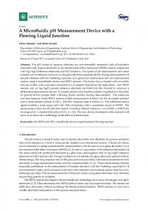
x/ac FIG. 1: A two-dimensional (x-y plane) sketch of our computational domain with the paths of two capsules, a stiff one (Ca = 0.05, solid blue line) and a floppy one (Ca = 0.3, broken red line), starting from the same initial position, at an offset hini = 0.015ac above the mid-plane (y = 0). The flow is driven from left to right. The diffuser (the diverging duct) makes an angle of 45◦ with the x axis. All length scales are normalized by the equilibrium radius, ac , of the capsule. The extent of the device in the z direction (perpendicular to the plane shown) is Hz = 4ac .

a function of only I1 = λ21 + λ22 − 2 and I2 = λ21 λ22 − 1, which are the two invariants constructed from the two principal components of the strain, λ1 and λ2 . Among several possibilities we choose the oft-used neo-Hookean model [16] for which   Gs 1 W = I1 − 1 + , (1) 2 I2 + 1 where Gs is the isotropic shear modulus. Another commonly used alternative is the Skalak model, used e.g., in Refs. 17, 18 for RBCs; see also Ref. 19 for a comparison between several constitutive models. We also employ a linear isotropic model for the bending moment, [20] with a bending modulus Gb = Cb a2c Gs , where ac is the radius of the capsule and Cb = 0.01 is held constant in our simulations. The choice of Cb is consistent with the available experimental data for RBCs. [12] Finally we also assume that the fluid inside and outside the cell has exactly the same density and viscosity; and the equilibrium shape of the cell is a sphere of radius ac . The model is specifically designed for anucleate cells, since the presence of a stiff nucleus is not explicitly considered. In spite of this fact, the model is potentially applicable to nucleate cells when the elastic constants, e.g., Gs , are tuned to effectively account for the internal cellular structures. To summarize, we solve for capsules with neo-Hookean membrane in flows. Even stripped of all its biological context, this problem is interesting in its own right for its potential applications to the fields of chemical engineering, bioengineering, and food processing among others.

There are two dimensionless numbers in this problem, the Reynolds number, Re ≡ ρU ac /µ, and the capillary number, Ca ≡ µU/Gs , where U is the characteristic velocity, µ the dynamic viscosity and ρ the density. The capillary number expresses the ratio between the viscous and elastic forces, which increases if the shear modulus decreases (softer capsules), or equivalently, if the mean velocity increases (larger fluxes). Hence, our results can be interpreted as either the dynamics of capsules with different deformabilities in the same flow, or that of the same capsule under different flow conditions. The Reynolds number is typically below 0.01 in microfluidic devices by virtue of the small length scales involved. Hence we use the linear Stokes equations (Re = 0) to solve the flow. For the sake of completeness, we provide a short description of the numerical algorithm [12, 22, 27] we use. The surface of the capsule is discretized into N points; the j-th point has the coordinate xj . In the spirit of immersed boundary methods; [23] at the j-th point, a force fj is exerted on the flow. These forces are determined by the deformation of the capsule with respect to its equilibrium shape through an appropriate constitutive law; in this case the neo-Hookean model. We use a spectral method [20] to calculate fj given the positions xj . The flow field can then be obtained by solving the Stokes problem, with the forces fj added to the right hand side, i.e., − ∇p + µ∇2 u = −

N X

fj δ (x − xj ) ,

(2)

j=1

∇ · u = 0.

(3)

Here p is the pressure, u is the velocity, and δ denotes the Dirac delta function. Equations 2 and 3 are solved by a hybrid IntegralMesh method. [24, 25] In our implementation, the meshbased part (responsible for the long-range part of the Green’s function) is calculated by the spectral-element solver NEK5000 [26] which allows us to cope with nontrivial boundaries. The short-range part is handled by standard boundary integral techniques. Once the Stokes problem is solved we know the velocity of the flow at every point including each point on the surface of the capsule, xj ; u(xj ). The values of xj at the next time step are obtained by solving, dxj = u(xj ). dt

(4)

This implies that the j-th point on the surface of the cell moves with the velocity, u(xj ), i.e., a no-slip, nonpenetrating boundary condition is satisfied on the cell surface. With this algorithm, we are able to perform high-fidelity simulations of deformable capsules suspended in microfluidic flows with complex domains. [27]

3 RESULTS

by: [29]   ∂W λ1 ∂W + λ22 , λ2 ∂I1 ∂I2   λ2 ∂W ∂W = 2 + λ21 . λ1 ∂I1 ∂I2

τ1P = 2 The device we propose is a rectangular duct attached to a diverging one (a diffuser), as shown in Fig. 1. An obstacle which encompasses the entire depth of the device (z direction), is positioned at the junction of the duct and the diffuser symmetrically about the mid-plane (y = 0). A capsule, whose equilibrium shape is a sphere of radius ac , is placed at the inlet. Initially, the centre of the capsule is not on the mid-plane but is displaced (along the y-direction) by an amount hini . The analytical flow profile [28] of a rectangular duct is maintained at the inlet, extreme left inFig. 1, and zero-stress boundary condi T tions −pI + µ ∇u + (∇u) = 0 are imposed at the outlet, extreme right in Fig. 1. The width and thickness of the duct (the extent of the y and z direction) is 8ac and 4ac , respectively; non-penetrating, no-slip boundary conditions are imposed on the wall of the device. The functioning of the device is demonstrated by a series of images in Fig. 2, see also the animation showing the motion of the capsules through our device at the location http : //www.youtube.com/watch?v = −1N bqQ GpSs. The flow field in the absence of the capsule is plotted in Fig. 2(a). When the capsule is at the inlet, the flow is very similar to that without the capsule. As the capsule approaches the obstacle, it slows down, deforms significantly (the deformation depends on Ca) and substantially modifies the flow as shown in Fig. 2(a)(f). Due to the interaction between the elastic membrane and the viscous flow, the capsules follow different paths depending on their deformability. Two extreme cases are sketched in Fig. 1 which demonstrate that at the outlet of the device two capsules with Ca = 0.05 (stiff) and 0.3 (floppy) are clearly separated. This completes our primary objective, i.e., to demonstrate that our device can sort capsules by deformability. The deformed shapes of the capsules for Ca = 0.05 (stiff) and Ca = 0.3 (floppy) at different positions along their trajectories are shown in Fig. 3. When the capsule passes around the obstacle, it blocks the flow and enhances the flow velocity on the opposite side of the obstacle; clearly, a stiffer (smaller Ca) capsule produces a stronger blockage. The deformation of the capsules are accompanied by large changes in their surface area as shown in the inset of Fig. 4. Note that, the fractional change of the area of the capsules is roughly proportional to their capillary number as can be seen from the collapsed curves shown in Fig. 4. The elastic stresses on the surface of the capsule are given by the two principal tensions, τ1P and τ2P , defined

τ2P

(5)

P The time evolution of the maximum stress, τmax , which P P is the maximum value of τ1 and τ2 calculated over the surface of the cell, is shown in Fig. 5 for three capillary numbers, Ca = 0.05, 0.2, and 0.3. The stress is maximum when the capsules pass through the gap and increases with Ca; for Ca = 0.3 it can be as large as 3.5 times Gs . Clearly, too strong mechanical stresses can rupture capsules although rupturing depends not only on the maximum value of the stress but also on how long it is applied. For example, RBCs at room temperature can even survive stresses up to 5000 Pascals for a very short time. [30] The time evolution of the maximum stress in Fig. 5 determines the type of cells that can be sorted in this device. The basic working principle of this device is the following. To distinguish capsules by deformability we apply an external flow that forces the capsules to pass through a narrow gap. The path of each capsule is then determined by the interaction between the viscous stresses and the elastic stresses; a relative measure of these two is the capillary number, Ca. For capsules with large Ca the viscous stresses dominate over the elastic ones, hence the trajectories of their centre-of-mass are close to the flow streamlines; these capsules deform far from their equilibrium shape. As an illustration, consider the limit Gs → ∞, Ca = 0. In this limit, the membrane of the capsule does not resist deformation and its material points (xj s) are advected by the flow as Lagrangian points. Consequently their centre of mass follows the streamline of the underlying flow. In contrast, capsules with smaller Ca deform less and can alter the flow more, hence their paths deviate further from the underlying flow; i.e., their centres are deflected further from the obstacle. The fact that a stiff capsule stays further from the obstacle than a soft one can also be understood in analogy with the collision of two capsules with different deformability. It has been shown that stiff capsules are displaced more than soft ones in heterogeneous collisions. [31, 32] If the obstacle is regarded as a capsule with infinitely large stiffness, it follows, according to these previous observations, that the distance between the obstacle and a moving capsule decreases with its deformability. The basic working principle of our device is the same as that of the Deterministic Lateral Displacement (DLD) devices. [11] In all cases, the variation in the trajectories after passing around a single obstacle is much smaller than the radius of the capsule, ac . Hence, by merely driving the capsules through a narrow gap (between the obstacle and the duct-walls) it is not possible to gener-

4 (a)

(b)

−4 −5

0

5

y/ac

0

x/ac

0

x/ac

5

−4

Ca=0.3 (floppy)

y/ac

0

−5

0

x/ac

5

−5

0

(d)

5

0

−5

0

5

0

5

x/ac

4

−4 x/ac

0

−4

4

0

−5

4

−4

4

−4 −5

0

y/ac

y/ac

4

4 y/ac

Underlying flow

y/ac

4

(c)

y/ac

Ca=0.05 (stiff)

0

−4 0

x/ac

(e)

5

−5

x/ac

(f)

FIG. 2: Two-dimensional profiles of two capsules at different time instants, plotted on the z = 0 plane with flow streamlines. The plot in the dashed box displays the streamlines of the flow without capsules. The evolution of the stiff capsule Ca = 0.05 and the floppy one Ca = 0.3, is illustrated in the top and bottom row respectively. The centre of mass of the capsule is indicated by the cross, and its trajectory by the dashed line. Snapshots are taken for each capsule at three time instants when: (a)/(d), the capsule almost touches the obstacle; (b)/(e), it sits in the gap above the obstacle; (c)/(f), it is well past the obstacle.

ate large enough differences between their trajectories to separate them. The DLD device [11] overcomes this limitation by using an array of obstacles to generate an accumulative outcome. We solve this problem by adding the diffuser where small displacements are magnified. The Pinched Flow Fractionation devices [33], which sort particles by their size, also use a diffuser. So far they have not been used to sort capsules by their deformability. Note that the presence of obstacle is essential to achieve sorting. Removing the obstacle, capsules with different deformability follow very close trajectories as shown by additional simulations for capillary numbers Ca = 0.05, 0.3, and offset hini = 0.15, 0.3. Let us now discuss the typical length scales involved in designing this device. In the sketch shown in Fig. 1 all the length scales have been normalized by ac . The radius of the obstacle is 2ac . The gaps through which the capsules pass have a width of 2ac too. Although the exact values of these sizes are not crucial, they must be of the same order of the size of the cells. Symmetry dictates that, if initially the capsule is placed exactly on the mid-plane it would get stuck in front of the obstacle, in the absence of thermal fluctuations. Estimates show that thermal fluctuations can be ignored in this problem. [12] Even without Brownian fluctuations, in an experimental realization, it would cer-

tainly be impossible that all the capsules are placed near the inlet with a precise initial offset, hini , from the midplane. How do small changes in hini affect the sorting capability of our device? To answer this question we run simulations for a range of values of Ca, each with several different values of hini . Let us concentrate on the stiffest capsule, Ca = 0.05, and the most floppy one, Ca = 0.3. If they are released from the same initial offset (hini ) then at the outlet the vertical displacement between their centres is larger than their diameter (2ac ), i.e., they are clearly separated, as shown in Fig. 1. Such a clear separation is not achieved if the capsules are released from different hini s. For example, the trajectories for the two cases, hini = 0.3, Ca = 0.3 and hini = 0.15, Ca = 0.05, are such that at the outlet the exit regions for the two cases overlap, see Fig. 6(a). To estimate this overlap, we plot, in Fig. 6(b), the displacements of the centre of the capsules from the mid-plane (at the outlet), ∆y, as a function of Ca, for hini = 0.15 and 0.3. The overlap between the capsules in Fig. 6(a) corresponds to the shaded region in Fig. 6(b). Figure 6(b) can be similarly used to calculate the overlap between any two points in the figure. Figure 6(b) clearly shows that the paths of floppy capsules (larger Ca) are more affected by the change in hini . Note that, the overlap is quite small compared to ac and can be reduced by using a longer diffuser.

5 (A)

(B)

(C) 3 2

1 Ca (A/A0 − 1)

2.5

0

1 E 2 max

Emax

Ca=0.3

1.8

2

1.6

Ca=0.2

1.4

1.5

1.2

1

Ca=0.05

1 0

10

5

15

0.5 0 0

10

5

20

15

t/tflow

To further understand how crucially the performance of this device depends on its design, we remove its spanwise confinement and impose periodic boundary conditions along the z direction; the results are plotted in Fig. 6 with the label “unconfined”. As expected, the absence of the spanwise confinement implies that for the same value of Ca, the vertical displacement decreases, in other words, the sorting capability of the device becomes weaker. Note that this comparison is made with the mean velocity of the underlying flow being held fixed. Next, instead of a perfect semi-cylindrical post, we test two more obstacles with semi-elliptic cross sections, made by stretching the semi-cylinder in the x direction by a factor of ξ = 2 and ξ = 2/3. Their cross sections are then two semi-ellipses with a major axis along the x and y direction, respectively. We find that the displacements between capsules with different deformability are essentially not altered by this geometric change, there is however a minor improvement in the sorting capability when the major axis is oriented along the x direction (ξ = 2). Finally, to understand the effects of the non-spherical shape of real biological cells, e.g., the bi-concave shape of RBCs, we investigate an initially oblate capsule. Its

4 Ca=0.3

3 P τmax /Gs

FIG. 3: Shapes of the capsule, with the computational grid sketched on the surface, at different instances during its passage through the device. Top row: Ca = 0.05. Bottom row: Ca = 0.3. At a time when (A) the capsule almost touches the obstacle, (B) the capsule sits in the gap between the obstacle and the duct-walls, (C) the capsule has gone well past the obstacle. The pseudocolors show the variation of the local strain energy function non-dimensionalized by Gs a2c ; E ≡ W/(Gs a2c ). Each plot is normalized by the maximum value of E, Emax . In the top row, Ca = 0.05, Emax = 0.04 (A), 0.1 (B), 0.004 (C). In the bottom row, Ca = 0.3, Emax = 0.47 (A), 3 (B), 0.07 (C).

FIG. 4: Fractional change in the surface area of the capsule, A/A0 − 1, for Ca = 0.05 (circle), 0.2 (square), and 0.3 (triangle) as a function of the nondimensionalized time t/tflow , where tflow ≡ ac /U . When the vertical axis is scaled by 1/Ca the three different curves collapse. The inset shows the unscaled case. The area of the capsule in its equilibrium configuration is A0 = 4πa2c .

2

1

0 0

Ca=0.2

Ca=0.05

5

10

15

20

t/tflow FIG. 5: The maximum value of the principal tension (EquaP tion (5)), nondimensionalized by Gs , τmax /Gs as a function of time for Ca = 0.05 (black filled circles), 0.2 (red squares), and 0.3 (blue triangles).

axes along the revolution axis and orthogonal directions are denoted by arc and aoc respectively and their ratio arc /aoc = 1/1.2; the volume is taken to be the same as the spherical capsules considered above. Two cells with Ca = 0.05 and Ca = 0.3 are simulated, with revolution axes initially oriented in the y direction. The displacement between the two cells at the outlet of the device decreases only by about 0.5% when compared to that between spherical capsules. Note that RBCs are oblates with an aspect ratio of around 3, and they can tumble in shear flows [14]. In such cases, the performance of our

6

y/ac

6

(a)

4 2 0−8

−4

0

4

5

12

16 18

(b)

4

y/ac

8

x/ac

3

2

1 0

0.1

0.2 Ca

0.3

0.4

FIG. 6: (a) Trajectories for Ca = 0.05 (stiff, red) and Ca = 0.3 (floppy, blue) for two initial offsets hini = 0.15 (solid) and 0.3 (dashed). The profiles of the capsules, at the outlet, clearly show an overlap. (b) The displacements of the centre of the capsules (∆y), above the mid-plane, measured at the outlet as a function of Ca for hini = 0.15 (solid) and hini = 0.3 (dashed). The vertical axis is normalized by the equilibrium radius of the capsule, ac . To calculate the overlap (the shaded region), for the pair of points Ca = 0.05, hini = 0.3 (red filled circle) and Ca = 0.3, hini = 0.15 (blue filled square), we draw circles of unit radius with the centres of the capsules as their respective origins. The overlap for any pair of points can be calculated in a similar manner. The dashed-dotted line with the symbol asterisk (∗) corresponds to the ”unconfined” case where we use periodic boundary conditions along the z direction.

device may deteriorate as the cell motion is not only affected by the deformability but also by the orientation of cells when approaching the obstacle.

CONCLUSIONS

We model cells as fluid-filled capsules enclosed by neoHookean membranes characterized by two elastic moduli, the shear modulus Gs and the bending modulus Gb ; the ratio between the two is held constant. Depending on the type of targeted cells, this model needs to be calibrated with the elastic measurements performed on the partic-

ular cells. For human RBCs, different methods, e.g., the measurements by micro-pipette [35] or that by optical tweezers [36, 37] give slightly different values of Gs . Diseases, e.g., sickle cell anaemia, can change this elastic coefficient by a factor of two to three, [38] and malaria can change the same elastic coefficient by a factor about ten. [2] This is consistent with the range of capillary number studied here. If we take a representative value of Gs ≈ 2.5µN/m [2], and use water as our fluid, then a typical flow rate of 0.1µlitre-per-minute gives Ca ≈ 0.06 which is well within the operating range of our device. We do not know the performance of the new device as the capillary number is outside the range we have studied; further work will be undertaken accordingly. As the sorting behaviour depends on Ca and not on Gs alone, the same device can be used in a different range of Gs values by merely changing the flow rate. A future direction is thus to investigate the sensitivity of the proposed mechanisms to inertial effects as the flow rate is much higher. To compare against other cell-sorting devices, the throughput of this device will be of the same order as that of the optical flow cytometers [1] because we can only allow one cell at a time to pass through the device. Margination devices [6] have a higher throughput as they operate on very many cells simultaneously, but the accuracy of the device we propose is expected to be significantly higher. We further note that optical flow cytometers can be modified to sort by deformability too by adding obstacles in the path of the cells and by optical recognition of their deformation. Due to the relatively simple model of the cell membrane used, and the fact that possible surface interactions between the cells and the walls of the device have been ignored, we do believe that further refinements of the suggested devices are possible. This work is the first numerical study of cell sorting in a realistic microfluidic device and shows how accurate simulations may guide the initial stages of the design of new devices. We hope that our work will inspire the experimental realization of devices based on the mechanism presented.

ACKNOWLEDGEMENTS

The work has been financially supported by grants from the Swedish Research Council (to CR and DM), the G¨oran Gustafsson foundation (CR) and the European Research Council, Advanced Grant, AstroDyn (DM). We thanks A. Brandenburg, R. Eichhorn and particularly D. Paul for many helpful discussions on possible experimental realization of the device. DM thanks IIT-B for hospitality, where a part of this work was carried out. Computer time provided by SNIC (Swedish National Infrastructure for Computing) is gratefully acknowledged. We thank the anonymous referee for pointing out the

7 possible limitations of our device in sorting highly nonspherical cells.

[1] P. Prasad, Introduction to Biophotonics, John Wiley and Sons, 2003. [2] S. Suresh, J. Mater. Res., 2006, 21, 1871–1877. [3] C. Lim and D. Hoon, Phys. Today, 2014, 67, 26. [4] X. Mao and T. Huang, Lab Chip, 2012, 12, 4006–4009. [5] R. Mebius and G. Kraal, Nature, 2005, 5, 606. [6] H. W. Hou, A. A. S. Bhagat, A. G. L. Chong, P. Mao, K. S. W. Tan, J. Y. Han and C. T. Lim, Lab Chip, 2010, 10, 2605–2613. [7] H. Bow, I. V. Pivkin, M. Diez-Silva, S. J. Goldfless, M. Dao, J. C. Niles, S. Suresh and J. Han, Lab Chip, 2011, 11, 1065–1073. [8] S. H. Holm, J. P. Beech, M. P. Barret and J. O. Tegenfeldt, Lab Chip, 2011, 11, 1326–1332. [9] S. C. Hur, N. K. Henderson-MacLennan, E. R. B. McCabe and D. D. Carlo, Lab Chip, 2011, 11, 912–920. [10] D. Gossett, T. Henry, S. Lee, Y. Ying, A. Lindgren, O. Yang, J. Rao, A. Clark and D. D. Carlo, Proc. Natl. Acad. Sci. U.S.A., 2012, 109, 7630–7635. [11] J. P. Beech, S. H. Holm, K. Adolfsson and J. O. Tegenfeldt, Lab Chip, 2012, 12, 1048–1051. [12] J. Freund, Annu. Rev. Fluid Mech., 2014, 46, 67–95. [13] Z. Peng, X. Li, I. Pivkin, M. Dao, G. Karniadakis and S. Suresh, Proc. Natl. Acad. Sci. USA, 2013, 110, 13356– 13361. [14] R. Finken, S. Kessler and U. Seifert, J. Phys-Condens. Mat., 2011, 23, 184113. [15] D. Barth`es-Biesel, Curr. Opin. Colloid. In, 2011, 16, 3– 12. [16] D. Barthes-Biesel, J. Walter and A.-V. Salsac, Computational hydrodynamics of capsules and biological cells, CRC Press, 2010. [17] J. Freund and M. Orescanin, J. Fluid Mech., 2011, 671, 466–490.

[18] J. Freund, Phys. Fluids, 2013, 25, 110807. [19] D. Barthes-Biesel, A. Diaz and E. Dhenin, J. Fluid Mech., 2002, 460, 211–222. [20] H. Zhao, A. H. G. Isfahani, L. N. Olson and J. B. Freund, J. Comput. Phys., 2010, 229, 3726–3744. [21] C. Pozrikidis, Phys. Fluids, 2005, 17, 031503. [22] L. Zhu and L. Brandt, J. Fluid Mech., 2013, submitted, null. [23] R. Mittal and G. Iaccarino, Annu. Rev. Fluid Mech., 2005, 37, 239–261. [24] A. Kumar and M. Graham, J. Comput. Phys., 2012, 231, 6682–6713. [25] J. Hern´ andez-Ortiz, J. de Pablo and M. Graham, Phys. Rev. Lett., 2007, 98, 140602. [26] P. Fischer, J. Lottes and S. Kerkemeier, nek5000 Web page, 2008, http://nek5000.mcs.anl.gov. [27] L. Zhu, PhD thesis, Royal Institute of Technology, KTH, 2014. [28] M. Spiga and G. Morino, Int. Commun. Heat Mass Transfer, 1994, 21, 469–475. [29] R. Skalak, A. Tozeren, R. P. Zarda and S. Chien, Biophys. J., 1973, 13, 245–264. [30] M. Musielak, Clin Hemorheol Micro, 2009, 42, 47–64. [31] A. Kumar and M. Graham, Phys. Rev. E, 2011, 84, 066316. [32] A. Kumar and M. Graham, Phys. Rev. Lett., 2012, 109, 108102. [33] M. Yamada, M. Nakashima and M. Seki, Anal. Chem., 2004, 76, 5465–5471. [34] P. G. Saffman and M. Delbr¨ uk, PNAS, 1975, 72, 3111. [35] X. Liu, Z. Tang, Z. Zeng, X. Chen, W. Yao, Z. Yan, Y. Shi, S. H, D. Sun, D. He and Z. Wen, Math. Biosci., 2007, 209, 190. [36] S. He` non, G. Lenormand, A. Richert and F. Gallet, Biophys. J, 1999, 76, 1145. [37] G. Lenormand, S. He` non, A. Richert, J. Sime´ on and F. Gallet, Biophys. J, 2001, 81, 43. [38] H. Lei and G. E. Karniadakis, Biophys. J, 2012, 102, 185.