simulation-based design methodology for CT Sigma-Delta modulators from high ... Circuit & Layout Level. Parasitics. Extraction. Layout. Design OK ! SNR, BW, OSR,. Technology. CAIRO+ ..... Power Spectral Density (dB) ideal. Aint1=0.216.
A Mixed Equation-Based and Simulation-Based Design Methodology For Continuous-Time Sigma-Delta Modulators H. Aboushady, L. de Lamarre, N. Beilleau and M.M Louerat University of Paris VI, LIP6/ASIM Laboratory, 4, Place Jussieu, 75252 Paris, France
Abstract— This paper presents a design automation tool for continuous-time Sigma-Delta modulators from high level specifications down to Layout. System level synthesis, circuit synthesis as well as layout synthesis are performed in the CAIRO+ design environment. Strong interaction between the system level and the circuit level is used to optimize the final design. The design of a complete third order currentmode continuous-time Sigma-Delta modulator is taken as an example to show the effectiveness of the proposed design methodology.
DT coeff, DAC Signal Shape
SNR, BW, OSR, Technology CAIRO+ Design Environment
DT-to-CT Transform
Scaling
Circuit Synthesis ( Sizing & Layout ) )
Σ∆
Parasitics Extraction
Reduce 1st Integrator Output Swing
CT Σ∆ Simulator
Circuit Simulator
I. Introduction Interesting work has been presented on the high level synthesis of Discrete-Time (DT) Σ∆ modulators for optimal topology selection and behavioral modeling of circuit non-idealities [1]. Top-down design methodologies from high level specifications down to layout for DT Σ∆ modulators have also been presented in [2][3]. Recently, Continuous-Time (CT) Σ∆ modulators are receiving increasing attention in high speed and low-power applications [4]. In this paper, we present a mixed equation-based and simulation-based design methodology for CT Sigma-Delta modulators from high level specifications down to Layout. The calculation and scaling of the Sigma-Delta coefficients as well as circuit sizing and layout generation are implemented in the same analog design environment CAIRO+. As can be seen from Figure 1, this has the important advantage to allow strong interaction between the different design levels. Here, we focus mainly on the interaction between the system-level and the circuit-level. A mixed equation-based and simulation-based design methodology is used to implement the tool. The paper is organized as follows. In Section II., systemlevel synthesis is presented. In section III., we present the circuit level design of the CT current-mode integrator, the current steering feedback DAC and the current comparator. Simulation-based circuit optimization is discussed in section IV.. Section V. is about layout synthesis. The conclusion is given in section VI..
Comparison
Circuit & Layout Level
System Level
Fig. 1. CT Σ∆ modulator synthesis in the CAIRO+ design environment.
Σ∆ loop gain Gc (z) is equal to the DT Σ∆ loop gain Gd (z). This can be expressed by
Gd (z) = Gc (z)
(1)
Gd (z) = Z [Hc (s) HDAC (s)]
A systematic technique for DT-to-CT transformation, based on the modified-z-transform technique, is then used to get the CT Σ∆ coefficients [5]. The complete procedure used to calculate the coefficients of a CT Σ∆ modulator, having an arbitrary feedback signal, is described in Figure 4. Using a symbolic mathematical tool, it is possible to obtain the CT coefficients (a1 , a2 , . . . , an ) expressed in function of the DT coefficients (b1 , b2 , . . . , bn ) and the 2
2
−gcn−1 2
− gc1
X(s) −
1 sT
1 sT
1 sT
1 sT
1 sT
an an−1
1 T U(s) U(z)
an−2 a3 a2
II. System-level synthesis
a1
A. Equation-based synthesis of CT Σ∆ coefficients To calculate the coefficients of continuous-time Σ∆ modulators, we start from the coefficients of a DT Σ∆ modulator. Figures 2 and 3 show general forms of a CT Σ∆ modulator and its DAC feedback signal, respectively. The objective is to design the CT loop filter Hc (s), for a given feedback DAC transfer function HDAC (s), so that the CT
H (s) DAC
Fig. 2. General form of a continuous-time Σ∆ modulator. td 1
0
τ
T
2T
3T
Fig. 3. Continuous-time rectangular feedback signal.
Y(z)
VDD
Σ∆ Topology CIFF, CRFF, ...
Calculate DT Loop Filter
Feedback Signal Characteristics td , τ , ...
Order n
Calculate Feedback DAC Transfer Function
Calculate CT Loop Filter
Vbias
M888
M88
M8
M7
M77
M777
Vcp
M666
M66
M6
M5
M55
M555
ion
Hd (z)
Hc (s)
iop
H (s)
inp
DAC
Vbc
Calculate DT Loop Gain
Calculate CT Loop Gain (modified-z-transform)
Gd (z)
Gc (z)
M444
M44
M222
M22
inn M4
M3
M2
M1
C
M33
M333
M11
M111
C
VSS
Compare Numerator and Denominator Coefficients
Fig. 6. The current-mode integrator.
...
a1 = f (b1 , b2 , ... , bn-1 , bn , td , τ, ...) a2 = f (b1 , b2 , ... , bn-1 , bn , td , τ, ...) an-1= f (b1 , b2 , ... , bn-1 , bn , td , τ, ...) an = f (b1 , b2 , ... , bn-1 , bn , td , τ, ...)
Fig. 4. Design procedure to find CT Σ∆ coefficients (a1 , . . . , an ) in function of DT Σ∆ coefficients (b1 , . . . , bn ) and the feedback signal characteristics (td , τ, . . . ).
feedback signal characteristics (td , τ, . . .): a1 = f (b1 , b2 , . . . , bn−1 , bn , td , τ, . . .) a2 = f (b1 , b2 , . . . , bn−1 , bn , td , τ, . . .) .. .
(2)
an−1 = f (b1 , b2 , . . . , bn−1 , bn , td , τ, . . .) an = f (b1 , b2 , . . . , bn−1 , bn , td , τ, . . .)
Symbolic DT-to-CT Σ∆ transformation tables are then obtained for different Σ∆ topologies, cascade of integrators or resonators in a feedforward or a feedback form.
Since the Σ∆ modulators are non-linear systems, simulation is usually involved in the design procedure. In the CAIRO+ environment, functions have been developed in order to perform simulation of ideal CT Σ∆ modulators. Functions for Fast Fourier Transform (FFT) and Signal to Noise Ratio (SNR) calculation are also available for the analysis of the output signal. The coefficients resulting from the DT-to-CT transformation tables, described in section A., ensure that both Noise Transfert Functions (NTF) of the DT and CT systems are identical. On the other hand, these coefficients do not take into account any circuit limitations. These coefficients do not ensure that the integrators outputs are 1 T
1/f1 sT
f1 /f2 sT
fi−1 /fi
1 / fn
sT
sT
Y(z)
an
1. the starting value for all the scaling factors is 1, f1 = f2 = . . . = fn = 1. 2. simulate the CT Σ∆ modulator with the previously determined scaling factor and the others left to 1, using a −6dB sinusoidal input signal. 3. the scaling factor, fi , corresponding to the ith simulation is calculated using the following expression:
B. Simulation-based scaling of CT Σ∆ coefficients
X(s)
limited to the maximum signal swing permitted by the circuit realizing the integrators. Due to the non-linearity of Σ∆ systems, the integrators output swing are difficult to predict mathematically and are then estimated by simulation. In [6], a systematic simulation-based technique to scale the CT Σ∆ coefficients for limited integrators output swing is presented. As seen in Figure 5, scaling factors (f1 , f2 , . . . , fn ) have been introduced to the CT Σ∆ system. These scaling factors are multiplied by the the CT Σ∆ coefficients and the integrators’ gains in such a way that the NTF is kept unchanged. The starting value for all the integrators’ gains and scaling factors is 1 and their final values will be determined by simulation using the following algorithm for an nth order modulator:
ai fi a2 f2 a1 f1
H (s) DAC
Fig. 5. Scaling factors are introduced to limit integrators output swing.
fi =
max(output ith integrator) desired ith integrator output swing
(3)
4. repeat steps 2 and 3 until i = n III. Equation-based circuit synthesis In this section, the design procedures used to synthesize the integrator, the feedback DAC and the comparator of the continuous-time Sigma-Delta modulator are presented. The biasing current and voltages are calculated using simplified MOS transistor models. The transistors’ dimensions are then calculated using the accurate BSIM3v3 models implemented in CAIRO+. A. Integrator Design Plan Figure 6 shows the fully differential current-mode integrator, taken here as a design example. Neglecting output conductances and parasitic capacitances, and assuming identical transistors, small-signal analysis of this circuit yields the following transfer function: Hcircuit (s) =
gm iinp (s) − iinn (s) = ioutp (s) − ioutn (s) sC
(4)
Fig. 8. DAC circuit. Fig. 7. Integrator synthesis procedure.
where gm is the transconductance of the mirror transistors M1 − M111 and M2 − M222 and C is the integrating capacitance. Figure 7, shows the design procedure used to size the transistors of the current-mode integrator. It has been shown in [7], that the maximum modulation index, , can be obtained using the following relation: m = IIin 0 √ √ 1 + m (VEG1 + VEG3 ) − 1 − m VEG1 − VT H 1 = 0 (5) where VEG1 and VEG3 are the effective gate voltages of the mirror transistor M1 and the cascode transitor M3 , respectively. The minimum integrating capacitance, C, necessary to achieve the desired SN R is calculated using the following equation [7]: C=
Ntr 4KT 8 SN R 2 2 3 AΣ∆ OSR Aint m2 VEG 1
(6)
the integrator gain, Aint , and the input signal gain for maximum SN R, AΣ∆ , are parameters calculated during the system level design. Ntr is the number of transistors contributing noise. The transfer function of each integrator in the Σ∆ modulator is determined during the system level design. This transfer function can be written in the following form Aint Hsystem (s) = sT
(7)
Comparing (7) and (4), it is obvious that for proper operation of the modulator the following relation must be satisfied: gm (8) Aint fs = C where fs = T1 is the sampling frequency of the modulator. The transconductance gm can also be written in the following form 2 I0 gm = (9) VEG By substitution from equation (9) into equation (8) we find that 2 I0 (10) Aint fs = VEG C Equation (10) is then used to calculated the biasing current I0 of the integrator. Using the BSIM3v3 sizing functions, we can generate a complete sized netlist of the integrator.
This integrator satisfies the required Signal-to-Thermal Noise ratio. On the other hand, this sizing procedure does not take the non-linearity of the integrator into account. The main source of harmonic distortion in the currentmode integrator, shown in Figure 6, is gm variation with the input current. It is possible to find an approximate expression for the transconductance gm (t) in function of the nominal transconductance gm0 , the input current iin (t), the biasing current I0 and the integrator gain Aint :
gm (t) = gm0
s
1+
Aint 1 I0 T
Z
t
iin (t) dt
(11)
0
From equation (11), we can see that it is possible to reduce the transconductance nonlinearity either by increasing the biasing current I0 or by decreasing the integrator gain Aint . In a low-power design, it is preferable to decrease the integrator gain Aint . If Aint is changed, all the coefficients of the Σ∆ modulator must be scaled in order to preserve the same NTF. Note that, although equation (11) is useful to identify the design parameters that influence the non-linearity of the integrator, it is very difficult to use this equation to estimate harmonic distortion of the CT Σ∆ modulator. B. Feedback DAC Design Plan Figure 8 shows the Feedback DAC circuit. Transistor M N1 acts as a current source and must be biased in deep saturation. Transistor M N2 acts as a switch and is biased in the linear region. M N5 is a cascode transistor biased in the saturation region. The biasing current IDACi is calculated in function of the integrator biasing current Ibias and the feedback coefficient, coefi , using the following relation: IDACi =
1 m Ibias coefi 2
(12)
Note the biasing voltages, should be given in function of the supply voltage or in function of other biasing voltages. This renders the design procedure independent from the technology and the desired specifications. Using the above information, the BSIM3v3 sizing functions are able to calculate the exact value of each transistor width.
VDD ckCOMP
VBIAS
VCP
VCP VOUT−
iIN +
−20
Power Spectral Density (dB)
VBIAS
0
VOUT+
VBC
iIN −
VBC
−40
−80
Circuit Simulator −100
−120
VSS
Harmonic Distortion
−60
CT SD Simulator
−140 −5 10
The current-mode comparator circuit is depicted in Figure 9. At its inputs, current mirrors, biased with the same current as the third integrator, copy the input signal to a clocked CMOS cross-coupled latch. IV. Simulation-based optimization Circuit simulation is used to measure harmonic distortion due to the non-linearity of the integrator circuit. The simulated circuit consists of a CT Σ∆ modulator using the sized netlist of the integrator (section A.) along with ideal models for the comparator and the feedback DAC. F F TREAL and SN RREAL calculations are performed on the simulation output. The CT Σ∆ simulator described in section B. is used to obtain F F TIDEAL and SN RIDEAL . The results of the system level simulation and circuit level simulation are compared. If SN RREAL < SN RIDEAL , the gain of the 1st integrator is reduced and the remaining coefficients are scaled in order to maintain the same NTF. Another circuit is then generated for the new coefficients. These steps are repeated until the difference between SN RREAL and SN RIDEAL is small. This optimization procedure is described in Figure 1. Figure 10 shows the results of such an optimization for a third-order continuous-time Σ∆ modulator. We can clearly see the large amplitude of the third harmonic for the first simulation done with coefficients scaled for maximum signal swing (Aint1 = 0.216). After several iterations, we find a suitable value (Aint1 = 0.043) which attenuates the third harmonic and gives an SN RREAL very close to SN RIDEAL . The main drawback of decreasing Aint is the corresponding increase in the integrating capacitance. V. Layout Synthesis In order follow a layout-aware approach for circuit synthesis [8], it is compulsory to be able to predict parasitics resulting from layout, early in the synthesis phase. Thus, we have chosen an approach using layout templates with dedicated layout device generators. The layout template which describes the relative placement of instances inside a circuit, is designed with the CAIRO+ language [9]. Device generators are available to the designer in the CAIRO+ environment. They can provide two types of information : layout and electrical information taking into account layout parasitics. These generators allow a given schematic to be ported to a new process or a new set of specifications.
−4
10
−3
10
−2
10
−1
10
0
10
Normalized Frequency (f / fs)
Fig. 9. Current-mode comparator.
C. Comparator Design Plan
ideal Aint1=0.216 Aint1=0.043
Fig. 10. Comparison between ideal system-level Σ∆ simulation and circuit level simulation.
VI. Conclusion A top-down design methodology of continuous-time Σ∆ modulators has been presented. The design methodology is mainly equation-based. Simulation is used in the system level to scale the calculated CT coefficients. In the circuit level, simulation is used to estimate harmonic distortion. It has been shown that circuit non-linearity can be reduced only by modifying the CT Σ∆ coefficients and without increasing the power consumption. Having almost all the calculations and simulations integrated in the same design environment, permitted strong interaction and optimization between the different design levels. References [1] K. Francken and G. Gielen. ”A High-Level Simulation and
[2]
[3]
[4]
[5]
[6]
[7]
[8]
[9]
Synthesis Environment for ∆Σ Modulators”. IEEE Transactions on Computer-Aided Design of integrated Circuits and Systems, vol. 22(No. 8):1049–1061, Aug. 2003. F. Medeiro, B. P´erez-Verd´ u, A. Rodr´ıguez-V´ azquez, and J. L. Huertas. ”A Vertically Integrated Tool for Automated Design of Σ∆ Modulators”. IEEE Journal of Solid-State Circuits, vol. 88(No. 12):762–772, July 1995. M. Dessouky, A. Kaiser, M. Lou¨erat, and A. Greiner. ”Analog Design for Reuse - Case Study: Very Low-Voltage ∆Σ Modulator”. IEEE Design Automation and Test in Europe Conference, pages 353–360, Mar. 2000. R. van Veldhoven, K. Philips, and B. Minnis. ”A 3.3mW Σ∆ modulator for UMTS in 0.18 µm CMOS with 70 dB dynamic range in 2 MHz bandwidth”. IEEE International Solid State Conference., Feb. 2002. H. Aboushady and M.-M. Lou¨erat. ”Systematic Approach for Discrete-Time to Continuous-Time Transformation of Σ∆ Modulators”. ISCAS, May 2002. N. Beilleau, H. Aboushady, and M.-M. Lou¨erat. ”Systematic Approach for Scaling Coefficients of Continuous-Time Sigma-Delta Modulators”. MWSCAS, Dec. 2003. H. Aboushady and M.-M. Lou¨erat. ”Low-Power Design of Low-Voltage Current-Mode Integrators for ContinuousTime Σ∆ Modulators”. ISCAS, May 2001. M. Dessouky, M. Lou¨erat, and J. Porte. ”Layout-Oriented Synthesis of High-Performance Analog Circuits”. IEEE Design Automation and Test in Europe Conference, pages 53– 57, Mar. 2000. P. Nguyen-Tuong, M.-M. Lou¨erat, and A. Greiner. ”Placement optimal d’objets d´eformables dans l’environnement de conception analogique CAIRO+”. Colloque CAO de circuits et syst`emes integr´es, http://asim.lip6.fr/gdrcao/articles, May 2002.