Based on these hypotheses, Wallis and Rolls produced a model of ventral ..... calculated by the following formula, with the details of the procedure given by Rolls ...
LETTER
Communicated by Laurenz Wiskott
A Model of Invariant Object Recognition in the Visual System: Learning Rules, Activation Functions, Lateral Inhibition, and Information-Based Performance Measures Edmund T. Rolls T. Milward Oxford University, Department of Experimental Psychology, Oxford OX1 3UD, England VisNet2 is a model to investigate some aspects of invariant visual object recognition in the primate visual system. It is a four -layer feedforward network with convergence to each part of a layer from a small region of the preceding layer, with competition between the neurons within a layer and with a trace learning rule to help it learn transform invariance. The trace rule is a modied Hebbian rule, which modies synaptic weights according to both the current ring rates and the ring rates to recently seen stimuli. This enables neurons to learn to respond similarly to the gradually transforming inputs it receives, which over the short term are likely to be about the same object, given the statistics of normal visual inputs. First, we introduce for VisNet2 both single-neuron and multiple-neuron information-theoretic measures of its ability to respond to transformed stimuli. Second, using these measures, we show that quantitatively resetting the trace between stimuli is not necessary for good performance. Third, it is shown that the sigmoid activation functions used in VisNet2, which allow the sparseness of the representation to be controlled, allow good performance when using sparse distributed representations. Fourth, it is shown that VisNet2 operates well with medium-range lateral inhibition with a radius in the same order of size as the region of the preceding layer from which neurons receive inputs. Fifth, in an investigation of different learning rules for learning transform invariance, it is shown that VisNet2 operates better with a trace rule that incorporates in the trace only activity from the preceding presentations of a given stimulus, with no contribution to the trace from the current presentation, and that this is related to temporal difference learning. 1 Introduction 1.1 Background. There is evidence that over a series of cortical processing stages, the visual system of primates produces a representation of objects that shows invariance with respect to, for example, translation, size, and view, as shown by recordings from single neurons in the temporal lobe c 2000 Massachusetts Institute of Technology Neural Computation 12, 2547–2572 (2000) °
2548
Edmund T. Rolls and T. Milward
(Desimone, 1991; Rolls, 1992; Rolls & Tovee, 1995; Tanaka, Saito, Fukada, & Moriya, 1991) (see Figure 2). Rolls (1992, 1994, 1995, 1997, 2000) has reviewed much of this neurophysiological work and has advanced a theory for how these neurons could acquire their transform-independent selectivity based on the known physiology of the visual cortex and self-organizing principles (see also Wallis & Rolls, 1997; Rolls & Treves, 1998). Rolls’s hypothesis has the following fundamental elements: A series of competitive networks, organized in hierarchical layers, exhibiting mutual inhibition over a short range within each layer. These networks allow combinations of features or inputs that occur in a given spatial arrangement to be learned by neurons, ensuring that higherorder spatial properties of the input stimuli are represented in the network. A convergent series of connections from a localized population of cells in preceding layers to each cell of the following layer, thus allowing the receptive-eld size of cells to increase through the visual processing areas or layers. A modied Hebb-like learning rule incorporating a temporal trace of each cell’s previous activity, which, it is suggested, will enable the neurons to learn transform invariances (see also Foldi´ ¨ ak, 1991). Based on these hypotheses, Wallis and Rolls produced a model of ventral stream cortical visual processing designed to investigate computational aspects of this processing (Wallis, Rolls, & Foldi´ ¨ ak, 1993; Wallis & Rolls, 1997). With this model, it has been shown that provided that a trace learning rule to be dened below is used, the network (VisNet) can learn transforminvariant representations. It can produce neurons that respond to some but not other stimuli with translation and view invariance. In investigations of translation invariance described by Wallis and Rolls (1997), the stimuli were simple stimuli such as T, L, and C , or more complex stimuli such as faces. Relatively few (up to seven) different stimuli, such as different faces, were used for training. The work described here investigates several key issues that inuence how the network operates, including new formulations of the trace rule that signicantly improve the performance of the network; how local inhibition within a layer may improve the performance of the network; how neurons with a sigmoid activation function that allows the sparseness of the representation to be controlled can improve the performance of the network; and how the performance of the network scales up when a larger number of training locations and a larger number of stimuli are used. The model described previously by Wallis and Rolls (1997) was modied in the ways just described to produce the model described here, which is denoted VisNet2. Before describing these new results, we rst outline the architecture of the model. In section 2, we describe a way to measure the performance of
Invariant Object Recognition in the Visual System
2549
the network using information theory measures. This approach has a double advantage: it is based on information theory, which is an appropriate measure for how any information processing system performs, and it uses the same measurement that has been applied recently to measure the performance of real neurons in the brain (Rolls, Treves, Tovee, & Panzeri, 1997; Rolls, Treves, & Tovee, 1997; Booth & Rolls, 1998), and thus allows direct comparisons in the same units, bits of information, to be made between the data from real neurons and those from VisNet. We then introduce the new form of the trace rule. In section 3, we show using the new information theory measure how the new version of the trace rule operates in VisNet and how the parameters of the lateral inhibition inuence the performance of the network; and we describe how VisNet operates when using larger numbers of stimuli than were used previously, together with values for the sparseness of the ring that are closer to those found in the brain (Wallis & Rolls, 1997; Rolls & Treves, 1998). 1.2 The Trace Rule. The learning rule implemented in the simulations uses the spatiotemporal constraints placed on the behavior of real-world objects to learn about natural object transformations. By presenting consistent sequences of transforming objects, the cells in the network can learn to respond to the same object through all of its naturally transformed states, as described by Foldi´ ¨ ak (1991) and Rolls (1992). The learning rule incorporates a decaying trace of previous cell activity and is henceforth referred to simply as the trace learning rule. The learning paradigm is intended in principle to enable learning of any of the transforms tolerated by inferior temporal cortex neurons (Rolls, 1992, 1995, 1997, 2000; Rolls & Tovee, 1995; Rolls & Treves, 1998; Wallis & Rolls, 1997). The trace update rule used in the simulations by Wallis and Rolls (1997) is equivalent to that of Foldi´ ¨ ak and the earlier rule of Sutton and Barto (1981), and can be summarized as follows:
D wj
t D ay .xj
where yt D (1 ¡ g)yt C gyt ¡1
xj :
j th input to the neuron.
yt :
Trace value of the output of the neuron at time step t .
wj :
Synaptic weight between j th input and the neuron.
y:
Output from the neuron.
a:
Learning rate; annealed between unity and zero.
g:
Trace value; the optimal value varies with presentation sequence length.
Edmund T. Rolls and T. Milward
Layer 4
Layer 3
Layer 2
Layer 1
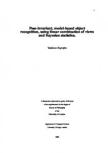
Figure 1: Stylized image of the VisNet four-layer network. Convergence through the network is designed to provide fourth-layer neurons with information from across the entire input retina.
To bound the growth of each cell’s dendritic weight vector, its length is explicitly normalized (Wallis & Rolls, 1997), as is common in competitive networks (see Rolls & Treves, 1998). 1.3 The Network. Figure 1 shows the general convergent network architecture used. The architecture of VisNet 2 is similar to that of VisNet, except that neurons with sigmoid activation functions are used, with explicit control of sparseness; the radius of lateral inhibition and thus of competition is larger, as specied below; different versions of the trace learning rule as described below are used; and an information-theoretic measure of performance replaces that used earlier by Wallis and Rolls (1997). The network itself is designed as a series of hierarchical, convergent, competitive networks, with four layers, specied as shown in Table 1. The forward connections to a cell in one layer come from a small region of the preceding layer dened by the radius in Table 1, which will contain approximately 67% of the connections from the preceding layer. VisNet is provided with a set of input lters that can be applied to an image to produce inputs to the network that correspond to those provided by simple cells in visual cortical area 1 (V1). The purpose is to enable within VisNet the more complicated response properties of cells between V1 and
Receptive Field Size / deg
2550
Invariant Object Recognition in the Visual System
2551
Table 1: VisNet Dimensions.
Receptive Field Size / deg
Layer 4 Layer 3 Layer 2 Layer 1 Retina
Dimensions
Number of Connections
Radius
32 £ 32 32 £ 32 32 £ 32 32 £ 32 128 £ 128 £ 32
100 100 100 272 —
12 9 6 6 —
50
TE
20
TEO
8.0
V4
3.2
V2
1.3
V1
view independence
view dependent configuration sensitive combinations of features
larger receptive fields
LGN 0 1.3 3.2 8.0 20 50 Eccentricity / deg Figure 2: Convergence in the visual system. V1: visual cortex area V1; TEO: posterior inferior temporal cortex; TE: inferior temporal cortex (IT). (Adapted from Rolls, 1992.)
the inferior temporal cortex (IT) to be investigated, using as inputs natural stimuli such as those that could be applied to the retina of the real visual system. This is to facilitate comparisons between the activity of neurons in VisNet and those in the real visual system to the same stimuli. The elongated orientation-tuned input lters used accord with the general tuning proles of simple cells in V1 (Hawken & Parker, 1987) and are computed by weighting the difference of two gaussians by a third orthogonal gaussian as described by Wallis et al. (1993) and Wallis and Rolls (1997). Each individual lter is tuned to spatial frequency (0.0625 to 0.5 cycles pixels¡1 over four C octaves), orientation (0–135 degrees in steps of 45 degrees), and sign (¡ 1). Of the 272 layer 1 connections of each cell, the number from each group is as shown in Table 2. Graded local competition is implemented in VisNet in principle by a lateral inhibition-like scheme. The two steps in VisNet were as follows. A local spatial lter was applied to the neuronal responses to implement
2552
Edmund T. Rolls and T. Milward
Table 2: VisNet Layer 1 Connectivity. Frequency Number of connections
0.0625
0.125
0.25
0.5
201
50
13
8
Note: The frequency is in cycles per pixel.
lateral inhibition. Contrast enhancement of the ring rates (as opposed to winner-take-all competition) was realized (Wallis and Rolls, 1997) by raising the ring P rates r to a xed power p, and then renormalizing the rates p (i.e., y D rp / ( i ri ), where y is the ring rate after the competition). The biological rationale for this is the greater than linear increase in neuronal ring as a function of the activation of the neuron. This characterizes the rst steeply rising portion close to threshold of the sigmoid-like activation function of real neurons. In this article, we introduce for VisNet2 a sigmoid activation function. The general calculation of the response of a neuron is as described by Wallis and Rolls (1997) and Wallis et al. (1993). In brief, the postsynaptic ring is calculated as shown in equation 2.1, where in this article the function f incorporates a sigmoid activation function and lateral inhibition, as described in section 2. The measure of network performance used in VisNet, the Fisher metric, reects how well a neuron discriminates between stimuli, compared to how well it discriminates between different locations (or more generally the images used rather than the objects, each of which is represented by a set of images, over which invariant stimulus or object representations must be learned). The Fisher measure is very similar to taking the ratio of the two F values in a two-way ANOVA, where one factor is the stimulus shown and the other factor is the position in which a stimulus is shown. The measure takes a value greater than 1.0 if a neuron has more different responses to the stimuli than to the locations. Further details of how the measure is calculated are given by Wallis and Rolls (1997). Measures of network performance based on information theory and similar to those used in the analysis of the ring of real neurons in the brain (see Rolls and Treves, 1998) are introduced in this article for VisNet2. They are described in section 2, compared to the Fisher measure at the start of section 3, and then used for the remainder of the article. 2 Methods 2.1 Modied Trace Learning Rules. The trace rule that has been used in VisNet can be expressed by equation 2.4, where t indexes the current trial and t ¡ 1 the previous trial. (The superscript on w indicates the version of the learning rule.) This is similar to Sutton and Barto (1981) and one of the formulations of Foldi´ ¨ ak (1991). The postsynaptic term in the synaptic
Invariant Object Recognition in the Visual System
2553
modication is based on the trace from previous trials available at time t ¡ 1 and on the current activity (at time t ), with g determining the relative proportion of these two. This is expressed in equation 2.3, where y is the postsynaptic ring rate calculated from the presynaptic ring rates xj as summarized in equation 2.1, and yt is the postsynaptic trace at time t . In this article, we compare this type of rule with a different type in which the postsynaptic term depends on only the trace left from previous trials available from t ¡ 1, without including a contribution from the current instantaneous activity y of the neuron. This is expressed in equation 2.5. In addition, we introduce a comparison of a trace incorporated in the presynaptic term (with the two variants for times t and t ¡ 1 shown in equations 2.6 and 2.7). The presynaptic trace, xjt , is calculated as shown in equation 2.2. We also introduce a comparison of traces incorporated in both the presynaptic and the postsynaptic terms (with the two variants for times t and t ¡ 1 shown in equations 2.8 and 2.9). We will demonstrate that using the trace at time t ¡ 1 is signicantly better than the trace at time t , but that the type of trace (presynaptic, postsynaptic or both) does not affect performance. What is achieved computationally by these different rules, and their biological plausibility, are considered in section 4. Following are these equations: yD f
±X
²
(2.1)
wj xj
xjt D (1 ¡ g)xjt C gxjt ¡1
(2.2)
y D (1 ¡ g)y C gy
(2.3)
t
D wj1 D wj2
t
yt xjt yt ¡1 xjt yt xjt
(2.4)
/
yt xjt ¡1 yt xjt C
(2.7)
/
yt ¡1 xjt C
/ /
D wj3 / D wj4
D wj5 / D wj6
t ¡1
(2.5) (2.6) yt xjt D D wj1 C D wj3 yt xjt ¡1
D
D wj2 C
(2.8)
D wj4
(2.9)
2.2 Measures of Network Performance Based on Information Theory.
Two new performance measures based on information theory are introduced. The information-theoretic measures have the advantages that they provide a quantitative and principled way of measuring the performance of an information processing system and are essentially identical to those that are being applied to analyze the responses of real neurons (see Rolls & Treves, 1998), thus allowing direct comparisons of real and model systems. The rst measure is applied to a single cell of the output layer and measures how much information is available from a single response of the cell
2554
Edmund T. Rolls and T. Milward
to each stimulus s. Each response of a cell in VisNet to a particular stimulus is produced by the different transforms of the stimulus. For example, in a translation-invariance experiment, each stimulus image or object might be shown in each of nine locations, so that for each stimulus there would be nine responses of a cell. The set of responses R over all stimuli would thus consist of 9NS responses, where NS is the number of stimuli. If there is little variation in the responses to a given stimulus and the responses to the different stimuli are different, then considerable information about which stimulus was shown is obtained on a single trial, from a single response. If the responses to all the stimuli overlap, then little information is obtained from a single response about which stimulus (or object) was shown. Thus, in general the more information about a stimulus that is obtained, the better is the invariant representation. The information about each stimulus is calculated by the following formula, with the details of the procedure given by Rolls, Treves, Tovee, and Panzeri (1997) and background to the method given there and by Rolls and Treves (1998): I (s, R ) D
X r2R
P (r | s) log2
P (r | s ) . P (r)
(2.10)
The stimulus-specic information, I (s, R), is the amount of information that the set of responses, R, has about a specic stimulus, s. The mutual information between the whole set of stimuli S and of responses R is the average across stimuli of this stimulus-specic information (see equation 2.11). (Note that r is an individual response from the set of responses R.) The calculation procedure was identical to that described by Rolls, Treves, Tovee, and Panzeri (1997) with the following exceptions. First, no correction was made for the limited number of trials, because in VisNet2 (as in VisNet), each measurement of a response is exact, with no variation due to sampling on different trials. Second, the binning procedure was altered in such a way that the ring rates were binned into equispaced rather than equipopulated bins. This small modication was useful because the data provided by VisNet2 can produce perfectly discriminating responses with little trial-to-trial variability. Because the cells in VisNet2 can have bimodally distributed responses, equipopulated bins could fail to separate the two modes perfectly. (This is because one of the equipopulated bins might contain responses from both of the modes.) The number of bins used was equal to or less than the number of trials per stimulus, that is for VisNet the number of positions on the retina (Rolls, Treves, Tovee, & Panzeri, 1997). Because VisNet operates as a form of competitive net to perform categorization of the inputs received, good performance of a neuron will be characterized by large responses to one or a few stimuli regardless of their position on the retina (or other transform), and small responses to the other stimuli. We are thus interested in the maximum amount of information that a neuron provides about any of the stimuli rather than the average amount
Invariant Object Recognition in the Visual System
2555
of information it conveys about the whole set S of stimuli (known as the mutual information). Thus, for each cell, the performance measure was the maximum amount of information a cell conveyed about any one stimulus (with a check, in practice always satised, that the cell had a large response to that stimulus, as a large response is what a correctly operating competitive net should produce to an identied category). In many of the graphs in this article, the amount of information that each of the 100 most informative cells had about any stimulus is shown. If all the output cells of VisNet learned to respond to the same stimulus, then the information about the set of stimuli S would be very poor and would not reach its maximal value of log2 of the number of stimuli (in bits). A measure that is useful here is the information provided by a set of cells about the stimulus set. If the cells provide different information because they have become tuned to different stimuli or subsets of stimuli, then the amount of this multiple cell information should increase with the number of different cells used, up to the total amount of information needed to specify which of the NS stimuli have been shown, that is, log2 NS bits. Procedures for calculating the multiple cell information have been developed for multiple neuron data by Rolls, Treves, and Tovee (1997) (see also Rolls & Treves, 1998), and the same procedures were used for the responses of VisNet. In brief, what was calculated was the mutual information I (S, R ), that is, the average amount of information that is obtained from a single presentation of a stimulus from the responses of all the cells. For multiple cell analysis, the set of responses, R , consists of response vectors comprising the responses from each cell. Ideally, we would like to calculate I (S, R ) D
X
P (s)I (s, R ).
(2.11)
s2S
However, the information cannot be measured directly from the probability table P (r, s) embodying the relationship between a stimulus s and the response rate vector r provided by the ring of the set of neurons to a presentation of that stimulus. (Note, as is made clear at the start of this article, that stimulus refers to an individual object that can occur with different transforms—for example, as translation here, but elsewhere view and size transforms. See Wallis and Rolls, 1997.) This is because the dimensionality of the response vectors is too large to be adequately sampled by trials. Therefore a decoding procedure is used in which the stimulus s0 that gave rise to the particular ring-rate response vector on each trial is estimated. This involves, for example, maximum likelihood estimation or dot product decoding. (For example, given a response vector r to a single presentation of a stimulus, its similarity to the average response vector of each neuron to each stimulus is used to estimate using a dot product comparison which stimulus was shown. The probabilities of it being each of the stimuli can be estimated in this way. Details are provided by Rolls, Treves, and Tovee
2556
Edmund T. Rolls and T. Milward
(1997) and by Panzeri, Treves, Schultz and Rolls (1999).) A probability table is then constructed of the real stimuli s and the decoded stimuli s0 . From this probability table, the mutual information between the set of actual stimuli S and the decoded estimates S0 is calculated as I (S, S0 ) D
X s,s0
P (s, s0 ) log2
P (s, s0 ) . P (s)P (s0 )
(2.12)
This was calculated for the subset of cells that had as single cells the most information about which stimulus was shown. Often ve cells for each stimulus with high information values for that stimulus were used for this. 2.3 Lateral Inhibition, Competition, and the Neuronal Activation Function. As originally conceived (Wallis & Rolls, 1997), the essentially
competitive networks in VisNet had local lateral inhibition and a steeply rising activation function, which after renormalization resulted in the neurons with the higher activations having very much higher ring rates relative to other neurons. The idea behind the lateral inhibition, apart from this being a property of cortical architecture in the brain, was to prevent too many neurons receiving inputs from a similar part of the preceding layer responding to the same activity patterns. The purpose of the lateral inhibition was to ensure that different receiving neurons coded for different inputs. This is important in reducing redundancy (Rolls & Treves, 1998). The lateral inhibition was conceived as operating within a radius that was similar to that of the region within which a neuron received converging inputs from the preceding layer (because activity in one zone of topologically organized processing within a layer should not inhibit processing in another zone in the same layer, concerned perhaps with another part of the image). However, the extent of the lateral inhibition actually investigated by Wallis and Rolls (1997) in VisNet operated over adjacent pixels. Here we investigate in VisNet2 lateral inhibition implemented in a similar but not identical way, but operating over a larger region, set within a layer to approximately half of the radius of convergence from the preceding layer. The lateral inhibition and contrast enhancement just described is actually implemented in VisNet2 in two stages. Lateral inhibition is implemented in the experiments described here by convolving the activation of the neurons in a layer with a spatial lter, I, where d controls the contrast and s controls the width, and a and b index the distance away from the center of the lter:
Ia,b D
8 2 2 ¡ a Cb > < ¡de s2 > :1 ¡
P
I 6 0 a,b aD 6 0 bD
6 0 or b D 6 0, if a D
if a D 0 and b D 0.
This is a lter that leaves the average activity unchanged.
Invariant Object Recognition in the Visual System
2557
Table 3: Sigmoid Parameters for the 25 Location Runs. Layer
1
2
3
4
Percentile
99.2
98
88
91
Slope b
190
40
75
26
The second stage involves contrast enhancement. In VisNet, this was implemented by raising the activations to a xed power and normalizing the resulting ring within a layer to have an average ring rate equal to 1.0. Here in VisNet2, we compare this to a more biologically plausible form of the activation function, a sigmoid, y D f sigmoid (r) D
1 , 1 C e¡2b (r¡a)
where r is the activation (or ring rate) of the neuron after the lateral inhibition, y is the ring rate after the contrast enhancement produced by the activation function, b is the slope or gain, and a is the threshold or bias of the activation function. The sigmoid bounds the ring rate between 0 and 1, so global normalization is not required. The slope and threshold are held constant within each layer. The slope is constant throughout training, whereas the threshold is used to control the sparseness of ring rates within each layer. The sparseness of the ring within a layer is dened (Rolls & Treves, 1998) as P ( yi / n ) 2 , a D Pi 2 i yi / n
(2.13)
where n is the number of neurons in the layer. To set the sparseness to a given value, for example, 5%, the threshold is set to the value of the 95th percentile point of the activations within the layer. (Unless otherwise stated here, the neurons used the sigmoid activation function as just described.) In this article we compare the results with short-range and longer-range lateral inhibition and with the power and activation functions. Unless otherwise stated, the sigmoid activation function was used with parameters (selected after a number of optimization runs), as shown in Table 3. The lateral inhibition parameters were as shown in Table 4. Where the power activation function was used, the power for layer 1 was 6 and for the other layers was 2 (Wallis & Rolls, 1997). 2.4 Training and Test Procedure. The network was trained by presenting a stimulus in one training location, calculating the activation of the neuron, then its ring rate, and then updating its synaptic weights. The sequence of locations for each stimulus was determined as follows. For a
2558
Edmund T. Rolls and T. Milward
Table 4: Lateral Inhibition Parameters for 25 Location Runs. Layer
1
2
3
4
Radius, s
1.38
2.7
4.0
6.0
Contrast, d
1.5
1.5
1.6
1.4
Figure 3: (Left) Contiguous set of 25 training locations. (Right) Five blocks of ve contiguous locations with random offset and direction.
value of g of 0.8, the effect of the trace decays to 50% after 3.1 training locations. Therefore, locations near the start of a xed sequence of, for example, 25 locations would not occur in sufciently close temporal proximity for the trace rule to work. The images were therefore presented in sets of, for example, 5 locations, with then a jump to, for example, 5 more locations, until all 25 locations had been covered. An analogy here is to a number of small saccades (or, alternatively, small movements of the stimulus) punctuated by a larger saccade to another part of the stimulus. Figure 3 shows the order in which (for 25 locations) the locations were chosen by sequentially traversing blocks of 5 contiguous locations, and visiting all 5 blocks in a random order. We also include random direction and offset components. After all the training locations had been visited (25 unless otherwise stated for the experiments described here), another stimulus was selected in a permutative sequence, and the procedure was repeated. Training in this way for all the stimuli in a set was one training epoch. The network was trained one layer at a time, starting with layer 1 (above the retina) through to layer 4. The rationale for this was that there was no point in training a layer if the preceding layer had a continually changing representation. The number of epochs per layer were as shown in Table 5. The learning rate was gradually decreasing to zero during the training of a layer according to a cosine function in the range 0 to p / 2, in a form of simulated annealing. The traceg value was set to 0.8 unless otherwise stated, and for the runs described in this article, the trace was articially reset to 0 between different stimuli. Each image was 64 £ 64 pixels and was shown at
Invariant Object Recognition in the Visual System
2559
Table 5: Number of Training Epochs per Layer. Layer
1
2
3
4
Number of epochs
50
100
100
75
different positions in the 128 £ 128 “retina” in the investigations described in this article on translation invariance. The number of pixels by which the image was translated was 32 for each move. With a grid of 25 possible locations for the center of the image as shown in Figure 3, the maximum possible shift of the center of the image was 64 pixels away from the central pixel of the retina in both horizontal and vertical directions (see Figure 3). Wrap-around in the image plane ensured that images did not move off the “retina”. The stimuli used (for both training and testing) were either the same set of 7 faces used and illustrated in the previous investigations with VisNet (Wallis & Rolls, 1997) or an extended set of 17 faces. One training epoch consists of presenting each stimulus through each set of locations, as described. The trace was normally articially reset to zero before starting each stimulus presentation sequence, but the effect of not resetting it was only mild, as investigated here and described below. We now summarize the differences between VisNet and VisNet2, partly to emphasize some of the new points addressed here, and partly for clarication. VisNet (see Wallis & Rolls, 1997) used a power activation function, only short-range lateral inhibition, the learning rule shown in equation 2.4, primarily a Fisher measure of performance, a linearly decreasing learning rate across the number of training trials used for a particular layer, and training that always started at a xed position in the set of exemplars of a stimulus. VisNet2 uses a sigmoid activation function that incorporates control of the sparseness of the representation and longer-range lateral inhibition. It allows comparison of the performance when trained with many versions of a trace learning rule shown in equations 2.5 through 2.9, includes information theory–based measures of performance, has a learning rate that decreases with a cosine bell taper over approximately the last 20% of the training trials in an epoch, and has training for a given stimulus that runs for several short lengths of the exemplars of that stimulus, each starting at random points among the exemplars, in order to facilitate trace learning among all exemplars of a given stimulus. 3 Results 3.1 Comparison of the Fisher and Information Measures of Network Performance. The results of a run of VisNet with the standard parameters
used in this article trained on 7 faces at each of 25 training locations are shown using the Fisher measure and the single-cell information measure in
2560
Edmund T. Rolls and T. Milward VisNet: 7f 25l: Single Cell Analysis trace hebb random
Fisher Metric
20 15 10 5 0
3
VisNet: 7f 25l: Single Cell Analysis trace hebb random
2.5 Information (bits)
25
2 1.5 1 0.5 0
10 20 30 40 50 60 70 80 90 100 Cell Rank Fisher Metric
10 20 30 40 50 60 70 80 90 100 Cell Rank Single Cell Information
Figure 4: Seven faces, 25 locations. Single cell analysis: Fisher metric and Information measure for the best 100 cells. Throughout this article, the single cell information was calculated with equation 2.10. Visnet: 7f 25l: Single Cell Analysis: Information v Fisher 3
Visnet: 7f 25l: Single Cell Analysis: Information v Fisher 3 2.5 Information (bits)
Information (bits)
2.5 2 1.5 1 0.5 0
2 1.5 1 0.5
0
2
4
6 8 10 12 14 16 18 Log Fisher Metric
0
0
0.5
1 1.5 2 2.5 Log Fisher Metric
3
3.5
Figure 5: Seven faces, 25 locations. Single cell analysis: Comparison of the Fisher metric and the information measure. The right panel shows an expanded part of the left panel.
Figure 4. In both cases the values for the 100 most invariant cells are shown (ranked in order of their invariance). (Throughout this article, the results for the top layer, designated 3, cells are shown. The types of cell response found in lower layers are described by Wallis & Rolls, 1997.) It is clear that the network performance is much better when trained with the trace rule than when trained with a Hebb rule (which is not expected to capture invariances) or when left untrained with what is random synaptic connectivity. This is indicated by both the Fisher and the single-cell information measures. For further comparison, we show in Figure 5 the information value for different cells plotted against the log (because information is a log measure) of the Fisher measure. It is evident that the two measures are closely related, and indeed the correlation between them was 0.76. This means that the information measure can potentially replace the Fisher measure because they provide similar indications about the network performance. An advantage of the information measure is brought out next. The information about the most effective stimulus for the best cells is seen (see Figure 4) to be in the region of 1.9 to 2.8 bits. This information measure
Invariant Object Recognition in the Visual System Visnet: 7f 25l: Cell (29, 31) Layer 3 ’face0’ ’face1’ ’face2’ ’face3’ ’face4’ ’face5’ ’face6’
Firing Rate
0.8 0.6 0.4 0.2 0
Visnet: 7f 25l: Cell (5, 30) Layer 3 1
’face0’ ’face1’ ’face2’ ’face3’ ’face4’ ’face5’ ’face6’
0.8 Firing Rate
1
2561
0.6 0.4 0.2
5
10 15 Location Index Information
20
0
5
10 15 Location Index Percentage Correct
20
Figure 6: Seven faces, 25 locations. Response proles from two top layer cells. The locations correspond to those shown in Figure 3, with the numbering from top left to bottom right as indicated.
species what perfect performance by a cell would be if it had large responses to one stimulus at all locations and small responses to all the other stimuli at all locations. The maximum value of the information I (s, R) that could be provided by a cell in this way would be log2 NS D 2.81 bits. Examples of the responses of individual cells from this run are shown in Figure 6. In these curves, the different responses to a particular stimulus are the responses at different locations. If the responses to one stimulus did not overlap at all with responses to the other stimuli, the cell would give unambiguous and invariant evidence about which stimulus was shown by its response on any one trial. The cell in the right panel of Figure 6 did discriminate perfectly, and its information value was 2.81 bits. For the cell shown in the left panel of Figure 6 the responses to the different stimuli overlap a little, and the information value was 2.13 bits. The ability to interpret the actual value of the information measure that is possible in the way just shown is an advantage of the information measure relative to the Fisher measure, the exact value of which is difcult to interpret. This, together with the fact that the information measure allows direct comparison of the results with measures obtained from real neurons in neurophysiological experiments (Rolls & Treves, 1998; Tovee, Rolls & Azzopardi, 1994; Booth & Rolls, 1998), provides an advantage of the information measure, and from now on we use the information measure instead of the Fisher measure. We also note that the information measure is highly correlated (r D 0.93) with the index of invariance used for real neuronal data by Booth and Rolls (1998). The inverted form of this index (inverted to allow direct comparison with the information measure) is the variance of responses between stimuli divided by the variance of responses within the exemplars of a stimulus. In its inverted form, it takes a high value if a neuron discriminates well between different stimuli and has similar responses to the different exemplars of each stimulus.
2562
Edmund T. Rolls and T. Milward VisNet: 7f 25l: Multiple Cell Analysis
2
100
trace hebb random
1.5
Percentage Correct
Information (bits)
2.5
1 0.5 0
5
10 15 20 Number of Cells Information
25
30
VisNet: 7f 25l: Multiple Cell Analysis
80
trace hebb random
60 40 20 0
5
10 15 20 Number of Cells Percentage Correct
25
30
Figure 7: Seven faces, 25 locations. Multiple cell analysis: Information and percentage correct. The multiple cell information was calculated with equation 2.12.
Use of the multiple cell information measure I (S, R ) to quantify the performance of VisNet2 further is illustrated for the same run in Figure 7. (A multiple cell assessment of the performance of this architecture has not been performed previously.) It is shown that the multiple cell information rises steadily as the number of cells in the sample is increased, with a plateau being reached at approximately 2.3 bits. This indicates that the network can, using its 10 to 20 best cells in the output layer, provide good but not perfect evidence about which of the 7 stimuli has been shown. (The measure does not reach the 2.8 bits that would indicate perfect performance mainly because not all stimuli had cells that coded perfectly for them.) Consistent with this, the graph of percentage correct as a function of the number of cells, available from the output of the decoding algorithm, shows performance increasing steadily but not quite reaching 100%. Figure 7 also shows that there is more multiple cell information available with the trace than with the Hebb rule or when untrained, showing correct operation of the trace rule in helping to form invariant representations. The actual type of decoding used, maximum likelihood or dot product, does not make a great deal of difference to the values obtained (see Figure 8), so the maximum likelihood decoding is used from now on. We also use the multiple cell measure (and percentage correct) from now on because there is no Fisher equivalent and because it is quantitative and shows whether the information required to identify every stimulus in a set of a given size is available (log2 NS ); because the percentage correct is available; and because the value can be directly compared with recordings from populations of real neurons. (We note that the percentage correct is not expected to be linearly related to the information, due to the metric structure of the space. See Rolls & Treves, 1998, section A2.3.4.) 3.2 The Modied Trace Learning Rule. A comparison of the different trace rules is shown in Figure 9. The major and very interesting performance difference found was that for the three rules that calculate the synaptic
Invariant Object Recognition in the Visual System VisNet: 7f 25l: Multiple Cell Analysis
2
90
1.5 1 0.5 0
VisNet: 7f 25l: Multiple Cell Analysis
80
trace opt trace dot hebb opt hebb dot random opt random dot
Percentage Correct
Information (bits)
2.5
2563
trace opt trace dot hebb opt hebb dot random opt random dot
70 60 50 40 30 20
5
10 15 20 Number of Cells Information
25
10
30
5
10 15 20 Number of Cells Percentage Correct
25
30
Figure 8: Seven faces, 25 locations. Multiple cell analysis: Information and percentage correct: Comparison of optimal (maximum likelihood) and dot product decoding. VisNet: 7f 25l: Single Cell Analysis pre (t) pre (t-1) both (t) both (t-1) post (t) post (t-1) random
Information (bits)
2.5 2 1.5 1 0.5 0
20
40
60 80 100 120 140 160 Cell Rank Single Cell
2.5
Information (bits)
3
VisNet: 7f 25l: Multiple Cell Analysis pre (t) pre (t-1) both (t) both (t-1) post (t) post (t-1) random
2 1.5 1 0.5 0
10
20 30 40 Number of Cells Multiple Cell
50
Figure 9: Seven faces, 25 locations. Comparison of trace rules. The three trace rules using the trace calculated at t ¡1 (labeled as pre(t ¡1) implementing equation 2.7, post(t ¡ 1) implementing equation 2.5 and both(t ¡ 1) implementing equation 2.9) produced better performance than the three trace rules calculated at t (labeled as pre(t) implementing equation 2.6, post(t) implementing equation 2.4, and both(t) implementing equation 2.8). Pre-, post-, and both specify whether the trace is present in the presynaptic or the postsynaptic terms, or in both.
modication from the trace at time t ¡ 1 (see equations 2.5, 2.7, and 2.9), the performance was much better than for the three rules that calculate the synaptic modication from the trace at time t (see equations 2.4, 2.6, and 2.8). Within each of these two groups, there was no difference between the rule with the trace in the postsynaptic term (as used previously by Wallis & Rolls, 1997), and the rules with the trace in the presynaptic term or in both the presynaptic and postsynaptic term. (Use of a trace of previous activity that includes no contribution from the current activity has also been shown to be effective by Peng, Sha, Gan, & Wei, 1998.) As expected, the performance with no training, that is, with random weights, was poor. The data shown in Figure 10 were for runs with a xed value ofg of 0.8 for layers 2 through 4. Because the rules with the trace calculated at t ¡1 might
Edmund T. Rolls and T. Milward
Max Info (bits)
2564
Visnet: 7f 25l 2.6 2.4 2.2 2 1.8 1.6 1.4 no reset (t) 1.2 reset (t) 1 no reset (t-1) reset (t-1) 0.8 0.6 0.55 0.6 0.65 0.7 0.75 0.8 0.85 0.9 0.95 1 Trace Eta
Figure 10: Seven faces, 25 locations. Comparison of trace rules, with and without trace reset, and for various trace values, g. The performance measure used is the maximum multiple cell information available from the best 30 cells.
have beneted from a slightly different value ofg from the rules using t , we performed further runs with different values of g for the two types of rules. We show in Figure 10 that the better performance with the rules calculating the trace using t ¡ 1 occurred for a wide range of values of g. Thus, we conclude that the rules that calculate the trace using t ¡ 1 are indeed better than those that calculate it from t and that the difference is not due to any interaction with the value of g chosen. Unless otherwise stated, the simulations in this article used a reset of the trace to zero between different stimuli. It is possible that in the brain, this could be achieved by a mechanism associated with large eye movements, or it is possible that the brain does not have such a trace reset mechanism. In our earlier work (Wallis & Rolls, 1997), for generality we did not use trace reset. To determine whether in practice this is important in the invariant representations produced by VisNet, in Figure 10 we explicitly compare performance with and without trace reset for a range of different values of g. It was found that for most values of g (0.6–0.9), whether trace reset was used made little difference. For higher values ofg such as 0.95, trace reset did perform better. The reason is that with a value of g as high as 0.95, the effect of the trace without trace reset will last from the end of one stimulus well into the presentations of the next stimulus, thereby producing interference by the association together of two different stimuli. Thus, with 25 presentations of each stimulus, trace reset is not necessary for good performance with values of g up to as high as 0.9. With 9 presentations of each stimulus, we expect performance with and without trace reset to be comparably good with a value of g up to 0.8. Further discussion of the optimal value and time course of the trace is provided by Wallis and Baddeley (1997). 3.3 Activation Function and Lateral Inhibition. The aim of this section is to compare performance with the sigmoid activation function introduced
Invariant Object Recognition in the Visual System
2565
for use with VisNet2 in this article with the power activation function as used previously (Wallis & Rolls, 1997). We demonstrate that the sigmoid activation function can produce better performance than the power activation function, especially when the sparseness of the representation in each layer is kept at reasonably high (nonsparse) values. As implemented, it has the additional advantage that the sparseness can be set and kept under precise control. We also show that if the lateral inhibition operates over a reasonably large region of cells, this can produce good performance. In the previous study (Wallis & Rolls, 1997), only short-range lateral inhibition (in addition to the nonlinear power activation function) was used, and the longer-range lateral inhibition used here will help to ensure that different neurons within the wider region of lateral inhibition respond to different inputs. This will help to reduce redundancy between nearby neurons. To apply the power activation function, the powers of 6,2,2,2 were used for layers 1 through 4, respectively, as these values were found to be appropriate and were used by Wallis and Rolls (1997). Although the nonlinearity power for layer 1 needs to be high, this is related to the need to reduce the sparseness below the very distributed representation produced by the input layer of VisNet. We aimed for sparseness in the region 0.01 through 0.15, partly because sparseness in the brain is not usually lower than this and partly because the aim of VisNet (1 and 2) is to represent each stimulus by a distributed representation in most layers, so that neurons in higher layers can learn about combinations of active neurons in a preceding layer. Although making the representation extremely sparse in layer 1, with only 1 of 1024 neurons active for each stimulus, can produce very good performance, this implies operation as a look-up table, with each stimulus in each position represented by a different neuron. This is not what the VisNet architecture is intended to model. Instead, VisNet is intended to produce at any one stage locally invariant representations of local feature combinations. Another experimental advantage of the sigmoid activation function was that the sparseness could be set to particular values (using the percentile parameter). The parameters for the sigmoid activation function were as in Table 3. It is shown in Figure 11 that with limited numbers of stimuli (7) and training locations (9), performance is excellent with both the power and the sigmoid activation function. With a more difcult problem of 17 faces and 25 locations, the sigmoid activation function produced better performance than the power activation function (see Figure 12), while at the same time using a less sparse representation than the power activation function. (The average sparseness for sigmoid versus power were: layer 1, 0.008 versus 0.002; layer 2, 0.02 versus 0.004; layers 3 and 4, 0.11 versus 0.015.) Similarly, with the even more difcult problem of 17 faces and 49 locations, the sigmoid activation function produced better performance than the power activation function (see Figure 13), while at the same time using a less sparse representation than the power activation function, similar to those just given.
2566
Edmund T. Rolls and T. Milward 3
Visnet: 7f 9l: Single Cell Information
3
Information (bits)
Information (bits)
2.5 2 1.5
sigmoid power
1
2.5 2
sigmoid power
1.5
0.5
1
0
0.5
0 100 200 300 400 500 600 700 800 900 Cell Rank Single Cell
Visnet: 7f 9l: Multiple Cell Information
5
10 15 20 Number of Cells Multiple Cell
25
30
Figure 11: Seven faces, 9 locations. Comparison of the sigmoid and power activation functions.
Information (bits)
3.5
Visnet: 17f 25l: Single Cell Information
2.5
sigmoid power Information (bits)
4
3 2.5 2 1.5 1 0.5
2
sigmoid power
1.5 1 0.5 0
10 20 30 40 50 60 70 80 90 100 Cell Rank Single Cell
Visnet: 17f 25l: Multiple Cell Information
5
10
15 20 Cell Rank Multiple Cell
25
30
Figure 12: Seventeen faces, 25 locations. Comparison of the sigmoid and power activation functions.
The effects of different radii of lateral inhibition were most marked with difcult training sets, for example, the 17 faces and 49 locations shown in Figure 14. Here it is shown that the best performance was with intermediaterange lateral inhibition, using the parameters for s shown in Table 4. These values of s are set so that the lateral inhibition radius within a layer is approximately half that of the spread of the excitatory connections from the
2
Visnet: 17f 49l: Single Cell Information
1.5 1 0.5 0
1.4
sigmoid power
Visnet: 17f 49l: Multiple Cell Information
1.2 Information (bits)
Information (bits)
2.5
1
sigmoid power
0.8 0.6 0.4 0.2
10 20 30 40 50 60 70 80 90 100 Cell Rank Single Cell
0
5
10 15 20 Number of Cells Multiple Cell
25
30
Figure 13: Seventeen faces, 49 locations. Comparison of the sigmoid and power activation functions.
Invariant Object Recognition in the Visual System Visnet: 17f 49l: Single Cell Analysis narrow medium wide
Information (bits)
1.6 1.4 1.2 1 0.8 0.6 0.4
10 20 30 40 50 60 70 80 90 100 Cell Rank Single Cell
Information (bits)
1.8
1 0.9 0.8 0.7 0.6 0.5 0.4 0.3 0.2 0.1 0
2567 Visnet: 17f 49l: Multiple Cell Analysis
narrow medium wide
5
10 15 20 Number of Cells Multiple Cell
25
30
Figure 14: Seventeen faces, 49 locations. Comparison of inhibitory mechanisms.
preceding layer. (For these runs only, the activation function was binary threshold. The reason was to prevent the radius of lateral inhibition affecting the performance partly by interacting with the slope of the sigmoid activation function.) Using a small value for the radius s (set to one-fourth of the values given in Table 4) produced worse performance (presumably because similar feature analyzers can be formed quite nearby). This value of the lateral inhibition radius is very similar to that used by Wallis and Rolls (1997). Using a large value for the radius (set to four times the values given in Table 4) also produced worse performance (presumably because the inhibition was too global, preventing all the local features from being adequately represented). With simpler training sets (e.g., 7 faces and 25 locations), the differences between the extents of lateral inhibition were less marked, except that the more global inhibition again produced less good performance (not illustrated). 4 Discussion
We have introduced a more biologically realistic activation function for the neurons by replacing the power function with a sigmoid function. The sigmoid function models not only the threshold nonlinearity of neurons, but also the fact that eventually the ring-rate of neurons saturates at a high rate. (Although neurons cannot re for long at their maximal ring rate, recent work on the ring-rate distribution of inferior temporal cortex neurons shows that they only rarely reach high rates. The ring-rate distribution has an approximately exponential tail at high rates. See Rolls, Treves, Tovee, & Panzeri, 1997, and Treves, Panzeri, Rolls, Booth, & Wakeman, 1999). The way in which the sigmoid was implemented did mean that some of the neurons would be close to saturation. For example, with the sigmoid bias a set at 95%, approximately 4% of the neurons would be in the high ringrate saturation region. One advantage of the sigmoid was that it enabled the sparseness to be accurately controlled. A second advantage is that it enabled VisNet2 to achieve good performance with higher values of the
2568
Edmund T. Rolls and T. Milward
sparseness a than were possible with a power activation function. VisNet (1 and 2) is, of course, intended to operate without very low values for sparseness. The reason is that within every topologically organized region, dened, for example, as the size of the region in a preceding layer from which a neuron receives inputs, or as the area within a layer within which competition operates, some neurons should be active in order to represent information within that topological region from the preceding layer. With the power activation function, a few neurons will tend to have high ring rates, and given that normalization of activity is global across each layer of VisNet, the result may be that some topological regions have no neurons active. A potential improvement to VisNet2 is thus to make the normalization of activity, as well as the lateral inhibition, operate separately within each topological region, set to be approximately the size of the region of the preceding layer from which a neuron receives its inputs (the connection spread of Table 1). Another interesting difference between the sigmoid and the power activation functions is that the distribution of ring rates with the power activation function is monotonically decreasing, with very few neurons close to the highest rate. In contrast, the sigmoid activation function tends to produce an almost binary distribution of ring rates, with most ring rates 0, and, for example, 4% (set by the percentile) with rates close to 1. It is this which helps VisNet to have at least some neurons active in each of its topologically dened regions for each stimulus. Another design aspect of VisNet2, modeled on cortical architecture, which is intended to produce some neurons in each topologically dened region that are active for any stimulus, is the lateral inhibition. In the performance of VisNet analyzed previously (Wallis & Rolls, 1997), the lateral inhibition was set to a small radius of 1 pixel. In the analyzes described here, it was shown, as predicted, that the operation of VisNet2 with longer-range lateral inhibition was better, with best performance with radii that were approximately the same as the region in the preceding layer from which a neuron received excitatory inputs. Using a smaller value for the radius (set to one-fourth of the normal values) produced worse performance (presumably because similar feature analyzers can be formed quite nearby). Using a large value for the radius (set to four times the normal values) also produced worse performance (presumably because the inhibition was too global, preventing all the local features from being adequately represented). The investigation of the form of the trace rule showed that in VisNet2, the use of a presynaptic trace, a postsynaptic trace (as used previously), and both presynaptic and postsynaptic traces produced similar performance. However, a very interesting nding was that VisNet2 produced very much better translation invariance if the rule used was with a trace calculated for t ¡ 1, for example, equation 2.5, rather than at time t , for example, equation 2.4 (see Figure 9). One way to understand this is to note that the trace rule is trying to set up the synaptic weight on trial t based on whether the neuron, based on its previous history, is responding to that stimulus (in
Invariant Object Recognition in the Visual System
2569
other positions). Use of the trace rule at t ¡ 1 does this, that is, takes into account the ring of the neuron on previous trials, with no contribution from the ring being produced by the stimulus on the current trial. On the other hand, use of the trace at time t in the update takes into account the current ring of the neuron to the stimulus in that particular position, which is not a good estimate of whether that neuron should be allocated to represent that stimulus invariantly. Effectively, using the trace at time t introduces a Hebbian element into the update, which tends to build positionencoded analyzers rather than stimulus-encoded analyzers. (The argument has been phrased for a system learning translation invariance but applies to the learning of all types of invariance.) A particular advantage of using the trace at t ¡ 1 is that the trace will then on different occasions (due to the randomness in the location sequences used) reect previous histories with different sets of positions, enabling the learning of the neuron to be based on evidence from the stimulus present in many different positions. Using a term from the current ring in the trace (the trace calculated at time t ) results in this desirable effect always having an undesirable element from the current ring of the neuron to the stimulus in its current position. This discussion of the trace rule shows that a good way to update weights in VisNet is to use evidence from previous trials but not the current trial. This may be compared with the powerful methods that use temporal difference (TD) learning (Sutton, 1988; Sutton & Barto, 1998). In TD learning, the synaptic weight update is based on the difference between the current estimate at time t and the previous estimate available at t ¡ 1. This is a form of error correction learning rather than the associative use of a trace implemented in VisNet for biological plausibility. If cast in the notation of VisNet, a TD(l) rule might appear as
D wj / (yt ¡ yt ¡1 )xjt ¡1 /
dt xjt ¡1 ,
(4.1) (4.2)
where dt D yt ¡ yt ¡1 is the difference between the current ring rate and the previous ring rate. This latter term can be thought of as the error of the prediction by the neuron of which stimulus is present. An alternative TD(0) rule might appear as
D wj / (yt ¡ yt ¡1 )xjt ¡1 / t
t d xjt ¡1 ,
(4.3) (4.4)
where d is a trace of dt the difference between the current ring rate and the previous ring rate. The interesting similarity between the trace rule at t ¡ 1 and the TD rule is that neither updates the weights using a Hebbian component that is based on the ring at time t of both the presynaptic
2570
Edmund T. Rolls and T. Milward
and postsynaptic terms. It will be of interest in future work to investigate how much better VisNet may perform if an error-based synaptic update rule rather than the trace rule is used. However, we note that holding a trace from previous trials, or using the activity from previous trials to help generate an error for TD learning, is not immediately biologically plausible without a special implementation, and the fact that VisNet2 can operate well with the ordinary trace rules (equations at time t) is important and differentiates it from TD learning. The results described here have shown that VisNet2 can perform reasonably when set more difcult problems than those on which it has been tested previously by Wallis and Rolls (1997). In particular, the number of training and test locations was increased from 9 to 25 and 49. In order to allow the trace rule to learn over this many variations in the translation of the images, a method of presenting images with many small and some larger excursions was introduced. The rationale we have in mind is that eye movements, as well as movements of objects, could produce the appropriate movements of objects across the retina, so that the trace rule can help the learning of invariant representations of objects. In addition, in the work described here, for some simulations the number of face stimuli was increased from 7 to 17. Although performance was not perfect with very many different stimuli (17) and very many different locations (49), we note that this particular problem is hard and that ways to increase the capacity (such as limiting the sparseness in the later layers) have not been the subject of the investigations described here. We also note that an analytic approach to the capacity of a network with a different architecture in providing invariant representations has been developed (Parga & Rolls, 1998). A comparison of VisNet with other architectures for producing invariant representations of objects is provided elsewhere (Wallis & Rolls, 1997; Parga & Rolls, 1998; see also Bartlett & Sejnowski, 1997; Stone, 1996; Salinas & Abbott, 1997). The results, by extending VisNet to use sigmoid activation functions that enable the sparseness of the representation to be set accurately, showing that a more appropriate range of lateral inhibition can improve performance as predicted, introducing new measures of its performance, and the discovery of an improved type of trace learning rule have provided useful further evidence that the VisNet architecture does capture and help to explore some aspects of invariant visual object recognition as performed by the primate visual system. Acknowledgments
The research was supported by the Medical Research Council, grant PG8513790 to E. T. R. The authors acknowledge the valuable contribution of Guy Wallis, who worked on an earlier version of VisNet (see Wallis & Rolls, 1997), and are grateful to Roland Baddeley of the MRC Interdisciplinary Research Center for Cognitive Neuroscience at Oxford for many helpful
Invariant Object Recognition in the Visual System
2571
comments. The authors thank Martin Elliffe for assistance with code to prepare the output of VisNet2 for input to the information-theoretic routines developed and described by Rolls, Treves, Tovee, and Panzeri (1997) and Rolls, Treves, and Tovee (1997); Stefano Panzeri for providing equispaced bins for the multiple cell information analysis routines developed by Rolls, Treves, and Tovee (1997); and Simon Stringer for performing the comparison of the information measure with the invariance index used by Booth and Rolls (1998).
References Bartlett, M. S., & Sejnowski, T. J. (1997). Viewpoint invariant face recognition using independent component analysis and attractor networks. In M. Mozer, M. Jordan, & T. Petsche (Eds.), Advances in neural information processing systems, 9. Cambridge, MA: MIT Press. Booth, M. C. A., & Rolls, E. T. (1998). View-invariant representations of familiar objects by neurons in the inferior temporal visual cortex. Cerebral Cortex, 8, 510–523. Desimone, R. (1991). Face-selective cells in the temporal cortex of monkeys. Journal of Cognitive Neuroscience, 3, 1–8. Foldi´ ¨ ak, P. (1991). Learning invariance from transformation sequences. Neural Computation, 3, 194–200. Hawken, M. J., & Parker, A. J. (1987). Spatial properties of the monkey striate cortex. Proceedings of the Royal Society, London [B], 231, 251–288. Panzeri, S., Treves, A., Schultz, S., & Rolls, E. T. (1999).On decoding the responses of a population of neurons from short time windows. Neural Computation, 11, 1553–1577. Parga, N., & Rolls, E. T. (1998). Transform invariant recognition by association in a recurrent network. Neural Computation, 10, 1507–1525. Peng, H. C., Sha, L. F., Gan, Q., & Wei, Y. (1998). Energy function for learning invariance in multilayer perceptron. Electronics Letters, 34(3), 292–294, Rolls, E. T. (1992). Neurophysiological mechanisms underlying face processing within and beyond the temporal cortical areas. Philosophical Transactions of the Royal Society, London [B], 335, 11–21. Rolls, E. T. (1994). Brain mechanisms for invariant visual recognition and learning. Behavioural Processes, 33, 113–138. Rolls, E. T. (1995). Learning mechanisms in the temporal lobe visual cortex. Behavioural Brain Research, 66, 177–185. Rolls, E. T. (1997). A neurophysiological and computational approach to the functions of the temporal lobe cortical visual areas in invariant object recognition. In L. Harris & M. Jenkin (Eds.), Computational and psychophysicalmechanisms of visual coding (pp. 184–220). Cambridge: Cambridge University Press. Rolls, E. T. (2000). Functions of the primate temporal lobe cortical visual areas in invariant visual object and face recognition. Neuron, 27, 1–20.
2572
Edmund T. Rolls and T. Milward
Rolls, E. T., & Tovee, M. J. (1995). Sparseness of the neuronal representation of stimuli in the primate temporal visual cortex. Journal of Neurophysiology, 73, 713–726. Rolls, E. T., & Treves, A. (1998).Neural networks and brain function. Oxford: Oxford University Press. Rolls, E. T., Treves, A., & Tovee, M. J. (1997). The representational capacity of the distributed encoding of information provided by populations of neurons in the primate temporal visual cortex. Experimental Brain Research, 114, 177–185. Rolls, E. T., Treves, A., Tovee, M., & Panzeri, S. (1997).Information in the neuronal representation of individual stimuli in the primate temporal visual cortex. Journal of Computational Neuroscience, 4, 309–333. Salinas, E., & Abbott, L. F. (1997). Invariant visual responses from attentional gain elds. Journal of Neurophysiology, 77, 3267–3272. Stone, J. V. (1996).A canonical microfunction for learning perceptual invariances. Perception, 25, 207–220. Sutton, R. S. (1988). Learning to predict by the methods of temporal differences. Machine Learning, 3, 9–44. Sutton, R. S., & Barto, A. G. (1981). Towards a modern theory of adaptive networks: Expectation and prediction. Psychological Review, 88, 135–170. Sutton, R. S., & Barto, A. G. (1998). Reinforcement learning. Cambridge, MA: MIT Press. Tanaka, K., Saito, H., Fukada, Y., & Moriya, M. (1991). Coding visual images of objects in the inferotemporal cortex of the macaque monkey. Journal of Neurophysiology, 66, 170–189. Tovee, M. J., Rolls, E. T., & Azzopardi, P. (1994). Translation invariance and the responses of neurons in the temporal visual cortical areas of primates. Journal of Neurophysiology, 72, 1049–1060. Treves, A., Panzeri, S., Rolls, E. T., Booth, M., & Wakeman, E. A. (1999). Firing rate distributions and efciency of information transmission of inferior temporal cortex neurons to natural visual stimuli. Neural Computation, 11, 611–641. Wallis, G., & Baddeley, R. (1997). Optimal unsupervised learning in invariant object recognition. Neural Computation, 9(4), 959–970. Available online at: ftp://ftp.mpik-tueb.mpg.de/pub/guy/nc.ps. Wallis, G., Rolls, E. T. (1997).A model of invariant object recognition in the visual system. Progress in Neurobiology, 51, 167–194. Wallis, G., Rolls, E. T., &Foldi´ ¨ ak, P. (1993). Learning invariant responses to the natural transformations of objects. International Joint Conference on Neural Networks, 2, 1087–1090. Accepted April 8, 1999; received November 24, 1998.