TRIBORS: A Triplet-Based Object Recognition System. Kari Pulli. 1 Introduction. Model-based object recognition 1] is a sub eld of Computer Vision that attempts ...
TRIBORS: A Triplet-Based Object Recognition System Kari Pulli
1 Introduction Model-based object recognition [1] is a sub eld of Computer Vision that attempts to deduce the identities and location of objects using sensor information. Typically, the sensor information comes in the form of a digitized camera image, where the data describes the intensity or color variations of the re ected light. Other sensors, such as laser range nders, are also possible sources of data. For recognition to be possible there rst has to be cognition; a system can only recognize an object if it has an internal representation against which the sensor data, or the features extracted from it, can be matched. The recognition system has often at its disposal some form of model, such as a CAD model, although ideally it should be able to build its own models by studying the objects or a set of typical images of the objects. Even in the cases that a good model is available, that model is probably not in the best format for solving the correspondence problem, i.e., for matching parts of the model to the sensor data. The correspondence problem can be tackled by studying the the interrelationships of features (see Vosselman [25] for a good description of relational matching). The mapping of model and object features is a combinatorial problem and is usually approached by applying some search method [10]. The Random Sample Consensus (RANSAC) [9] avoids the combinatorics of an exhaustive search by using a randomized hypothesis-veri cation method. The related Local Feature Focus (LFF) method [2] tries to constrain the large search space by concentrating on small clusters of key features. The 3DPO system [13] implements the same ideas in 3D using range data. Other techniques for making the expensive search more intelligent include nding viewpoint invariant features [15] [24] or perceptual groupings [19] [12] that can be used to constrain the possible mappings. There are two related methods for evaluating the partial or nal matches. One of them is based on information theory [3] [25], while the other is based on probability theory [4]. Our approach is the probabilistic one and is related to the PREMIO system of Camps [4]. PREMIO (Prediction in Matching Images to Objects) constructs view-dependent probability models that incorporate the errors due to the interplay of surface re ectance properties, lighting conditions, and image processing operators. The matching method used in PREMIO is an iterative-deepening A* search guided by probability information about feature attributes. The system described in this paper is called TRIBORS (Triplet-Based Object Recognition System). Like PREMIO, TRIBORS uses synthesized images to create probability models for matching. The main motivation for this research was to try out the ideas of the PREMIO system, provide a 1
projecting a wireframe
Create Probability Model: Create triplets, their para-
and using Eq. 3
meters and frequencies
Match image lines by
Create synthetic images
Prune the Probability Model
Obtain real images
Match objects using the Probability Model and
Match image and model lines using pose,
pose estimator (Eqs. 1&2)
wireframe and Eq. 3
Create new Probability Model and prune it
Figure 1: Creation of the Probability Model for matching. more robust implementation, remove several limitations of its current implementation, and test a di�erent matching method:
� In PREMIO all coordinates and angles describing features are expressed in absolute screen
� � � �
coordinates, so the system requires the objects to be centered and aligned with the vertical screen axis. In TRIBORS the features used for matching are triplets that are parameterized in a 2D a�ne invariant manner, so no particular screen location or orientation is preferred over others. PREMIO uses its own ray tracing routine, which is slow and hard to modify. TRIBORS generates synthetic images using a general ray tracer which allows more experimentation with lighting and feature extraction operators and is also signi cantly faster. Edge detection in PREMIO is done by the simple Sobel operator; TRIBORS uses the more robust Canny edge detector combined with the ORT line linker. TRIBORS does not rely only on synthetic images when building probability models for matching, but generates new models by using matched real images as the source of more accurate data. The current implementation of PREMIO does not verify the result of the matching and does not use all the available data for obtaining as accurate a pose 1 estimate as possible. Match veri cation and pose re ning are integral parts of the matching algorithm of TRIBORS.
Figure 1 shows the steps in creating a probability model for matching objects. We start by describing the feature triplets, the unit of matching that enables us to hypothesize the pose of the object. Then we explain the ideas behind the probability models. Next the matching method, a 1
Pose means the orientation and location.
2
hypothesize-verify method, is described. The system structure and its components are explained and the results are presented.
2 Feature triplets In this section we rst discuss the the local feature focus method to give the motivation for using a succinct set of features, such as line triplets, as the basis for matching. Then we compare our method to Heniko� and Shapiro's representative patterns, and nally we show how the line triplets can be parameterized in a way that is invariant to both rotations and translations on a plane.
De nition 1 A triplet T is a tuple T = (L1; L2; L3; P� ; P�) where L1, L2 and L3 are three noncollinear line segments, and P� and P� are the means and standard deviations, respectively, of the parameterization of T with respect to a view class V .
2.1 Local Feature Focus method A straightforward way for matching two sets of features, one set from a model and the other one extracted from an image, is to match one feature at a time, check whether the matched feature is consistent with all the previously matched features, and continue until no more consistent matches can be done. The largest set of matches whose elements are all pairwise consistent is chosen as the match. This algorithm is, however, equivalent to nding the maximal cliques in a graph, a problem which is known to be NP-complete. Often only a few matched features are enough to fully constrain the pose of the whole object, and hence also the locations of all the other features. This is the idea behind the Local Feature Focus (LFF) method of Bolles and Cain [2]. The method uses only small sets of features that are spatially close to each other for overcoming a common problem in object recognition: occlusion. If the object in the image is partially hidden by another object, or if some features are hidden by self-occlusion, or if part of the object is damaged or missing, the LFF method can still work. If a feature has been detected, it makes sense to search for features close to it, since they have a greater chance of also being visible. If enough features can be recovered the whole pose can be estimated and the match can be veri ed by projecting the model features onto the image and checking whether they match the features in the image. If the veri cation fails, the search process can be continued. Using features that are spatially close to one another does have the advantage of being more robust against occlusion, but using sets of spatially extended features usually gives better estimates of the pose of the object, especially in the 3D case, where the error tolerances for feature locations used by the pose estimation algorithm are much lower that in the 2D case. Thus it may be advantageous to use both spatially concise and spatially extended feature sets; triplets use both lines that are touching and lines that are widely separated. Triplet matching does not remove the need for searching, but it guarantees that the search space will never grow very large, since the depth of the search tree is limited to three, the number of features needed to constrain the object pose. 3
2.2 Representative patterns Heniko� and Shapiro [12] have presented a matching method based on based on representative patterns, a collection of edge chains consisting of sets of linked line segments. The building blocks of the edge chains are ordered sets of three lines called triples. The triples are not parameterized, the only requirements are that the three lines are adjacent and they have two concave junctions, so that the triple forms a \U" shape. Representative patterns are rst created from object models. The result is a graph, where the nodes correspond to triple chains and arcs correspond to relationships between pairs of chains. Similar graphs are formed from the edges extracted from the images and the graphs are matched using consistent labeling relaxation. Representative patterns is a symbolic approach to the object matching problem. The method yields candidates for matching image lines to object lines but it does not directly provide an accurate pose estimate or a veri cation of a hypothesized match. The lack of parameterization of the \U" triples has both advantages and disadvantages. The triples are very robust against perspective distortions and changes of appearance when rotated in 3D. On the other hand, this general characterization means that the triples cannot be matched in isolation, but only in context of several other triples, whose interrelationships are known. Since three line matches are enough in most cases to constrain the view point to a unique solution [6], 2 we chose to concentrate more on individual line triplets rather than tracking their relationships. Our triplets are not constrained to be joint, and their appearance is not constrained in any way. Individual line triplets are often formed from the edges, but virtual line triplets can be derived by drawing lines between triplets of points, centers of holes, corners, etc., as long as the features have a location.
2.3 Parameterizing line triplets To enable matching of line triplets in the absence of context information about other triplets we need to parameterize their shapes. A robust representation of the features and their combinations remains invariant even when a triplet is moved around or rotated on the image plane. The following parameterization of line triplets ful lls these requirements.
De nition 2 A parameterization P of a triplet T with respect to a view class V is a tuple P = (D; O), where D is a tuple of distance parameters D = fl1; l2; l3; d2; d3) and O is a tuple of orientation parameters O = ( 2; 3; �2; �3 ). Figure 2 shows the parameterization of a line triplet. One of the lines is chosen to be the basis line (the line with the arrow head), and all the distances and orientations are calculated relative to 2 Degenerate cases, such as when the lines lie close to a common 3D line, do not yield a reliable pose, but in most cases a unique pose estimate can be obtained.
4
2
l2
l3
3
d2
d3
�3 �2
l1
Figure 2: Parameterization of a line triplet. that. Three of the parameters, l1 , l2 and l3, represent the lengths of the lines, and two parameters, d2 and d3, represent the distances from the midpoint of the rst line to the midpoints of the two other lines. Two parameters, �2 and �3 , de ne the directions of the other lines' midpoints from the rst line. In order to disambiguate the directions, we have to de ne a direction for the rst line so that the midpoint of the second line lies counterclockwise from the rst line, i.e., �2 must be in the range of [0::� ). The third line can lie in any direction, i.e., �3 has range [0::2� ). The two remaining arguments, 2 and 3, denote the di�erence of the orientations of the second and third lines from the base line. For disambiguation this angle is restricted to (?�::0]3. This parameterization is now invariant to translation and orientation on the image plane. In order to be fully 2D a�ne invariant, the description needs to be also invariant with respect to scaling. This is achieved by dividing all the length parameters in D by the length of the base line l1.
3 Probability models In general, a probability model of an object contains information about the expected frequency of the object appearing in an image, about the frequencies of certain features appearing (assuming that the object appears in the image), and about the likely relations and attribute values of those features. In our system the probability model consists of a set of line triplets and the expected values and the standard deviations of the triplets' parameters. Those triplets that are least useful for matching will be discarded from the model.
De nition 3 A probability model M is a set of tuples (T ; pT ) where T is a triplet and pT is the probability of T being extracted from an image taken from some direction � 2 V , where V is the view class of the probability model M. In this section we rst discuss the information in a probability model for purposes of matching the model to an image. Next we brie y discuss view classes; the probability models in our system 3
[0; �) or (?�=2; �=2] would be ne as well.
5
are speci c for di�erent view classes. Then we will describe how we obtain the training data for calculating the statistics for the probability model. The data used for matching should rapidly produce good matches: we next describe how the data set is pruned. Last we will show how the re ning of a probability model can be viewed as a machine learning task.
3.1 The information in a probability model Our probability model contains information about the identities of features used for matching, information about the expected parameter values and their distributions and information about their frequency of appearance. The idea of calculating the frequencies of appearance of an object or of a feature is that we can penalize or disqualify an unlikely choice, either when creating the probability model or when matching an image against a model. If we have models for several objects or for several view classes of an object, we can associate a higher matching cost for the models that seldom appear. In the case that we have a great number of features in the probability model, we can prune the size of the model by discarding features or combinations of features that either seldom appear or are often matched incorrectly. So that we can match features, we need to know what they will look like, i.e., what are the expected values (means �) and the variations (standard deviations � ) of the parameters describing the features. These parameters give us a way of normalizing the di�erences in parameter values so they can be summed to give the cost of the t even though their ranges vary a lot. The distance of a parameter p from its expected value �p can be normalized by p0 =
j p ? �p j : �p
(1)
The various normalized distances can then be summed together to get the total cost of the t. Sometimes some of the parameters are deemed more relevant than the others, and one may want to be able to express the relative relevance by giving di�erent variables di�erent relative weights. In that case the total cost C (Fimage ; Fmodel ) of mapping image features Fimage to model features Fmodel becomes the weighted sum wi � p0i : (2) C (Fimage ; Fmodel ) =
X
pi 2Fmodel
3.2 View classes The shape of the projection of a 3D object to a 2D image plane varies a lot when the object is viewed from di�erent directions. Small changes in view point, however, do not normally change the appearance very much. From this fact arises the idea of view classes [23].
De nition 4 A view class is a set of views V , so that if �1; �2 2 V and Si is a structural description of the features visible from �i , i 2 f1; 2g, then F� (S1; S2) < � for some relational distance function F� and threshold �. 6
An informal de nition of a view class is a contiguous region of viewing directions such that differences in the appearance of features are small when looked at from di�erent directions within the region. It is possible that some faces or edges of an object are visible, or partially or totally occluded, depending on the exact view and the threshold �. The determination of the correct view class could be done by geometric hashing [24] where some salient features vote for the directions where they can be observed, or the application can be one where only a couple of di�erent view classes are possible. For example, an assembly part coming on a conveyer belt could have only a limited number of stable orientations. However, nding the correct view class is outside of the scope of this project. We assume that the view class has been either identi ed or hypothesized and we look for a a correct match and corresponding pose within a view class. Concentrating on a single view class at a time makes it possible to do the actual matching in 2D for 3D objects. The parameters can be calculated describing the projections of features and their interrelationships, and many of them will remain in relatively compact volumes of the parameter space. This is not true for all the feature combinations, but usually there are quite a few potential feature combinations, so the ones that greatly vary within a view class can be discarded. Once the matching has been done in 2D, we can calculate the pose of the object. Knowing the pose gives us a way of verifying the correctness of the matching using 3D knowledge: all the features can be projected to the image plane and we can check that the ones that should be visible are present in the image and the ones that should be invisible have not been matched.
3.3 Building the probability model The data needed for calculating the probability models can be obtained by taking sets of real images and analyzing them or by creating sets of synthesized views that cover the view class. We use both methods. The system is bootstrapped by creating synthetic images using a ray tracing and graphical modeling package. A description of the object is constructed, the colors and re ectivities of the surfaces are de ned, and the lighting is de ned. Then the ray tracer is called several times to create views from several viewing directions so that the view points cover the view class uniformly. In this phase we have the advantage that the view point is known; we do not have to match a whole 3D model, but only the 2D projections of the 3D lines against the extracted 2D lines. The matched lines are used in constructing the probability model. We compare three measures to determine the similarity of two lines:
� line lengths, � line orientations, and � the distance between the lines' midpoints. There do not exist meaningful values for means or standard deviations for these measures, and therefore it is up to the user to scale the di�erences or residuals. A good way to do this is to 7
de ne for each value a threshold for the residual to be too large for the lines to be considered similar. Then the three residuals will be scaled by dividing each residual by the corresponding threshold, and the results can be summed to a number that describes the similarity (the matching cost) of the two lines. If the lengths are denoted by �, angles by � 2 [0::� ) and distances by � , and the corresponding thresholds are �thr , �thr , �thr , respectively, the similarity measure or the cost C (L1; L2) for two lines L1 and L2 (such that �1 � �2 ) is C (L1; L2) =
j �1 ? �2 j + min(�1 ? �2; �2 + � ? �1) + �1!2 : �thr
�thr
�thr
(3)
We do not have to take any extra measures to model the errors and inaccuracies caused by the feature extracting operators, because the same operators will be used both to obtain the data for the probability model and in the actual matching. For example, if the edge detectors tend to round the corners or not nd short edges, the e�ects will be re ected in the data and will be incorporated into the probability model. Obtaining synthetic images that are very much like actual camera images is quite di�cult. The re ectance properties of the real objects are not quite uniform and simple to model even if the whole object is manufactured from the same material. The re ectance model of the graphics system may not be realistic enough; ray tracing is good in producing shadows and specular re ections, but it ignores di�use re ections, i.e., it uses a local rather than a global illumination model. Even if the graphics system takes care of the global illumination to various degrees of approximation (like the radiosity method does), the lighting conditions with ltered ood lights and indirect lighting may be di�cult to model. Regardless of the limitations, the synthetic images provide an approximation of the real data that is often good enough to produce probability models for matching real images. The actual probability models consist of a collection of model line triplets, the expected values for the parameters describing the projections of the model lines within a view class, and the standard deviations for the parameter values. Once we have a probability model we can match real images. Now it is possible to take several di�erent images from typical viewing directions within a view class at the application site with the existing lighting conditions and camera parameters. The images are analyzed and matched, the matches are veri ed and the recovered features are stored. The resulting data can be used to create a new probability model that better ts the conditions at the application site.
3.4 Pruning the probability model Not all the possible triplets of model lines are very useful in matching. It does not, for example, make much sense to use triplets that are totally or partially hidden when the object is viewed from view points within the view class. Other non-useful triplets are those whose lines lie close to a common 3D line; that kind of triplet would not give a good pose estimate. Additionally, since our triplet representation is not indi�erent to the ordering of the lines within the triplet, it makes sense to only include one of the six possible permutations. 8
We start creating the probability model by creating all the possible triplets. We calculate the frequency of appearance for each triplet (the probability term pT of Def. 3) by counting in how many training images all three lines of the triplet were detected. If that frequency is too low, the triplet is discarded. Similarly, the triplets whose model lines lie in the same 3D line will be discarded, since they are not likely to lead to good pose estimates. For each permutation of each remaining triplet, we calculate the means P� and standard deviations P� of the parameters. Since parameter sets with small standard deviations allow fewer false matches, we retain only the permutation whose squared sum of standard deviations is the smallest. For the remaining triplets and for all the images where all the lines of the triplet have been detected, we calculate the cost of tting the correct three lines. This is done by calculating the parameters P , normalizing with P� the di�erences from P� using Eq. 1 and summing them up using Eq. 2. Then, for each image, we calculate the costs of the ts for all possible line triplets created from the extracted lines and count how many false triplets, on the average, have a lower tting cost than the correct one. Salient features (triplets that are quite di�erent from the other possible triplets) tend to do well here: their tting cost is rather low compared to all other costs of tting random triplets. On the other hand, when there are random triplets within the view class that have similar parameters to a given triplet, that triplet is likely to do worse. Such undistinguished triplets are removed in this phase.
3.5 Probability models seen as machine learning problem The idea behind the probability models is to use the model of an object and a set of images (synthetic or real) of the object for creating search control data to expedite the matching process. This formulation enables us to look at the creation of probability models as an instance of explanationbased learning problem. Explanation-based learning [21] [22] enables an intelligent and economical use of training examples by using prior information. The method iterates over three steps: explanation, analysis, and re nement. Explanation. The rst step uses domain theory, in our case the CAD-model and the possible knowledge of the locations of light sources and camera locations, to explain that the current training example is indeed an instance of the modeled object, or more generally, of the target concept. Analysis. The second step analyzes the explanation to identify the features of the training example that enable the correct classi cation. This step is often intertwined with the explanation part: we reach the explanation as a result of analysis. This does not always have to be the case, since we could have an oracle (e.g., the user) that performs the classi cation, whereas the learning system has to derive the analysis by itself. Our case is kind of a mix: while creating the probability model we know that the object is going to appear in the synthetic image and then the system has to analyze the image to actually nd it. Re nement. The last step changes the search control rules by adding new rules that allow the recognition of the current instance. 9
Probability models in our system are created in a batch mode. Initially all we have is the CADmodel of an object and a set of synthetic images along with view parameters. The images allow the creation of the initial probability model. Although we tried to create the synthetic images as realistically as possible, they di�er from real images. It is easy to render the synthetic images so that all the model features can be easily detected; it is more di�cult, however, to render the images so that we will detect those and only those features that can be detected from real images. There are several reasons for this: the illumination model is not realistic enough, the actual camera is not really a pinhole camera and its blurring e�ects are di�cult to model, the re ectivity function of the object surface and the lighting conditions are only approximately known and their interaction cannot be accurately described by using only three (R, G, and B) samples of di�erent wavelengths, etc. When we start changing the parameters of the renderer so that the synthetic images would appear more realistic, it often happens that some features that can be obtained from real images cannot be found in the synthetic ones, and vice versa. Once we have a preliminary probability model from the synthetic images, we can use it to match real images. The matched features of the real images are more reliable and can be used to re ne the probability model or create it totally anew.
4 Matching Matching is the most important component of an object recognition system; other parts such as the probability model exist only to facilitate and expedite matching. Once the correct match has been established, the correspondence of model and image features can be used to obtain the pose of the object. On the other hand, the knowledge of the pose can help verify the correctness of the match. In general, the matching procedure must be able to di�erentiate between several possible objects, and if view classes are used, between several di�erent view classes. In this project, we assume that the object is known and the view class has been identi ed or hypothesized. Matching is thus the process of nding the correspondence between triplets of the image and triplets of the view class, estimating the pose of the object and verifying the match.
4.1 Matching the model triplets to the image features Our matching procedure begins with the extraction of edges from the input image. Having obtained a set of straight line segments, we choose a batch of a few triplets (seven in the current implementation) from our probability model and search for an image line triplet that most closely resembles the current model line triplet, i.e., has the lowest cost when tted to the current model triplet. Notice that an exhaustive search is not needed; we can calculate a subset of the attributes from two image lines, and if they contribute more to the matching cost of the current triple than 10
the costs of the best tting triplets found so far, we can skip all the triplets with those two image lines. The matching or tting cost is de ned by taking the absolute value of the di�erence of each triplet parameter value from the expected value. Since the di�erent parameters have di�erent types (some measure relative angles, others relative distances or lengths) and some parameters vary more than the others, the di�erences are not directly comparable. Therefore the di�erences are normalized and summed, using Eqs. 1 and 2. Because the line orientations can be recovered more accurately than the lengths, the orientation terms will receive greater weights wi in Eq. 2. Our matching method allows for changes in the scale, i.e., the observation distance can be greater or smaller than the distance used when the training set was created. This is achieved by calculating a scaling factor by averaging the individual ideal scaling factors of the di�erent parameters: 1 �a s= ; D = fl ; l ; l ; d ; d g: (4)
X
j D j a2D a
1
2 3
2
3
The scaling factor s is used as the weight wi for the distance parameters in Eq. 2, but the user can give the allowed range of s and hence determine the allowed distance range.
4.2 Initial pose estimation Once we have determined which image line triplets have a low matching cost against the model triplets, we hypothesize for each low cost match that it is the correct match. The next step is to obtain an initial estimate for the pose of the object. Dhome et al. [6] have developed a method that analytically derives the possible 3D poses from matched triplets of image lines by solving the inverse perspective equations. The problem is decomposed into two parts: the rst part solves the relative rotation or the orientation between the sensor and the object, and the second part solves for the translation or the location. Many other methods require a rough initial guess for the pose in order to converge to a solution. For example Lowe [19] [20] gave an iterative algorithm based on Newton's method that can be used for obtaining poses of parameterized 3D objects. Other methods are described in [16] and [14]. For our purposes we could use any of those methods, since the general viewing direction is assumed to be known by the choice of the probability model (there is a one-to-one correspondence between probability models and view classes). Our matching method does not depend on any particular pose estimation algorithm. Since we did not have an available implementation of the abovementioned algorithms (their implementation would have been a quite non-trivial task), but we did have access to an iterative point-to-point correspondence based algorithm described in section 5.1, we used what was readily at hand.
4.3 Match veri cation So far we have guessed the identity of an object and its pose based on a small set of features. Now we need to verify that hypothesis. The pose estimate we have allows us to predict locations of the 11
other object features by projecting the visible features of the object onto the image. The veri cation starts with the creation of a wireframe image of the object model so that the pose of the wireframe equals the initial pose estimate. The visibility of the edges of the wireframe can be determined by a hidden line detection algorithm [18]. Our system implements a quick version of that algorithm which removes most of the hidden lines. Once the visible edges and their locations have been predicted we search for image lines that would match them. We nd for each predicted edge the closest image line such that one image line can map to only one predicted edge and vice versa. The closeness is determined using the cost of tting a line to another, according to Eq. 3. A tting cost of less than 1.0 is considered a match.4 If the initial pose estimate was close to the correct pose, we can nd more matching lines in addition to the three from the current triplet. In that case the new line matches give more information to the pose estimator, and a new, more accurate estimate is obtained. This pose estimation - line matching cycle is iterated as long as we can match more line pairs. If the initial triplet match was wrong, we may still be able to match the three line pairs and maybe one or two more. In such a case the odds of nding several chance matching line pairs are very low, and the match can be discarded on the basis that only a couple of image lines support it. There are two gures on the basis of which we can determine the success of the match veri cation. One is the number of matched lines and the other is the sum of the tting costs for the line matches (obtained using Eq. 3).
5 Experiments 5.1 Software Our original goal was to reuse existing software modules as much as possible. Although several large modules could be reused, quite a lot more had to be written by the author (more than 4000 lines of C++ code). Synthesized images. The synthesized images used for creating data for the construction of the probability models were created by Rayshade, a public domain ray shading package. Rayshade provides a nice modeling language for creating object models. Di�erent lighting options are available (point lights sources, directed light, even area lights) and the defocusing and blurring of real camera images can be modeled by changing the aperture of the virtual camera lens and by blurring the resulting image using Gaussian or block lters. The biggest drawback in relation to our project is the local lighting model inherent in ray tracing methods: the ambient lighting is poorly modeled and the di�use inter-re ections between the object's surfaces is not modeled at all. The generated images model reality well if the lighting conditions are harsh: only a couple of strong spotlights used in an otherwise dark room. However, the best results when using real cameras (from the The cost function has three parts, distance, length, and angle, each producing 1.0 if the di�erence equals threshold. Thus if any of them di�ers by the threshold, or two of them di�er by half of the threshold, etc., the sum exceeds 1.0. 4
12
point of view of obtaining object features reliably) can be obtained using soft lighting with reduced shadows. Edge detection. We use the Canny edge detector [5] for extracting the edges from the images. The idea behind this detector is to rst calculate the gradients of the intensities within the image and then to link together pixels with high gradient values. The same programs are used for both the synthesized and the real images. Line detection. The edge pixels obtained using the Canny edge detector are input to the Object Recognition Toolkit (ORT) [7] [8] which extracts straight lines and circular arcs from the edgel chains. ORT also provides for grouping of the line segments according to parallel, collinear, intersecting, etc. relationships. Pose estimation. We use only one algorithm for obtaining both the initial estimate for the pose and for the re ned pose estimate. The exterior orientation algorithm, implemented by Ken Thornton and described in [11], needs as its input a set of 3D-point-to-2D-point (model-to-image) correspondences and a starting guess for the viewing parameters5. There are several ways of obtaining point correspondences from line correspondences. The simplest way is to match the end points of the lines. This is somewhat error prone: although the orientation and the location of the lines can be determined quite accurately, the edge detector tends to shorten the lines somewhat at the corners. One solution would be to approximate how much the extracted lines really are shorter than the actual lines in the image and grow the lines correspondingly. Another possibility arises if the 3D lines are known to intersect at some corner of the object: the image lines can be extended until they intersect on the screen. We chose a third option with more point to point correspondences, which gives more constraints to the pose estimation algorithm. Both the image lines and the model lines can be chopped into short sections, and the end points of the sections give more correspondences. Although equidistant sections of an image line do not strictly speaking correspond to equidistant sections of the corresponding model line because of the perspective distortion, the errors caused by the perspective projection are quite small. This is because the objects are usually far enough so that within the projected area of a single edge we can assume an orthogonal projection. The extra constraints for the pose estimator give better results than if they are not used (the end points have probably already more location error than the new points).
5.2 Testing environment The facilities of the testing environment, other than the computers and the software, consisted of a camera, video grabber, lamps, lters, and two metal objects. The camera was a Pulmix TM-7CN camera with a CCD-array of 494 � 768 elements. The focal length of the objective was 25 mm. The video grabber was by Data Translation and it converted the signal from the camera to a 512 � 480 digitized grey valued image. We had polarized lters both for the halogen lights and the objective 5 This particular algorithm was chosen over line based pose estimation algorithms because the implementation was available and the its author could be consulted when needed.
13
Figure 3: The test objects Fork and Cube3Cut. of the camera. Figure 3 shows the test objects. The larger one on the left is called Fork and the smaller one on the right is Cube3Cut.
5.3 Matching results For testing the matching algorithm we took 100 real camera images of Cube3Cut and Fork. The images form ve sets of 20 images that each form a view class: three classes for Cube3Cut and two classes for Fork. Figure 4 shows a typical view from each view class. Each image set is taken from a di�erent distance and contains 10 images. Within the 10-image sets the object is placed in a stable position and it is slightly manually rotated from image to image. (see Fig. 5)
Figure 4: Representative images from the ve view classes. Initially we have the bootstrapping problem: to be able to calculate the probability model that can be used to expedite matching, we need to have a set of matched images showing the line correspondences, and for obtaining that we need to either
� use a probability model (which we do not have) to speed up the search of correct match, � exhaustively search for correct line matches and verify the result (which would be really slow),
or � know the relative position and orientation between the camera and the object so we can project the model over the image. 14
Figure 5: The complete set of images for one of the view classes.
15
We do not know the accurate relative positions between the camera and the object in the real images. However, if we generate a set of images ourselves, we know the values of these parameters. After we project the edges of the object to these synthesized images, the nding of line correspondences is very easy. The viewing directions for the synthesized images were chosen so that they cover the view class approximately uniformly. The directions were represented in an object centered polar coordinate system. The user gives the maximum and minimum values for the latitude and longitude, and also the number of samples that will be taken. For example, the images for the rst view class of Cube3Cut were generated such that the object was rotated on the table (corresponds to the latitude) 10, 19, ... , and 55 degrees (6 steps), while the angle of the viewing direction and the positive z-axis was varied between 62, 69, and 76 degrees, producing altogether 18 synthesized images. Figure 6 (a) shows a typical synthesized image. The rst processing step for this image was to detect edges in that image (Fig. 6 (b)). The edge pixels were then linked into lines and arches as shown in Fig. 6 (c). Next each potentially visible line of the model was projected onto the line image using the known viewing parameters. If a line whose location, orientation, and length correspond closely enough to the projected line was found among the detected lines, a match was declared. Figure 6 (d) shows such lines.
(a)
(b)
(c)
(d)
Figure 6: (a) A synthesized image of Cube3Cut. (b) The lines extracted by the Canny operator. (c) The lines and arches extracted by the ORT routines. (d) The matched lines of the synthesized image. Notice that several of the visible edges could not be reliably extracted: the contrasts over the edges may have been low, and in a few cases the line detection algorithm broke an edge into two. The fact that we get results like this from synthesized images only goes to show that the matching algorithm needs to be robust against missing, and sometimes also erroneus data in order to work with real images that are bound to contain some amount of noise. Note also that all of the edge lines that were almost completely extracted were matched with line from the geometric model, while none of the false or partial lines were matched. Using the collection of matched lines from all the synthesized images within the view class a probability model consisting of parameterized triplets was created. This enabled us to actually 16
(a)
(b)
(c)
(d)
Figure 7: (a) The edges extracted from the real image. (b) The lines and arches extracted by the ORT routines. (c) The matched triplet (thick lines) and the initial pose estimate. (d) The nal match and pose. match real images, rst by nding potential matches based on triplet information, and then verifying the match while at the same time re ning the pose estimate of the object. The matching of triplets is done in a batch before we start verifying the triplet matches. We rst randomly select seven triplets from the probability model. Then we search for image line triplets that t well the current model triplet. We store seven best possible matches, which we then verify. Note that the stored triplet matches do not necessarily each come from a di�erent model triplet. This would happen if, for example, we nd two image line triplets matching the third model triplet of the batch such that their matching costs are less than the best triplet match of the second model triplet. In the case we cannot verify a match for any of the potential matches within a batch, we continue with a next batch; otherwise we have succeeded. Figure 7 presents the steps in matching the leftmost image of Fig. 4. Figure 7 (a) and (b) shows the results of edge detection and line linking, respectively. Notice that although the orientations of the real object and the synthesized are almost the same, and light comes from the same direction in both images, there are several edge lines detected in the synthetic image that were not detected in the real image, and conversely some (real) edge lines in the real image that were not detected in the synthetic image. Figure 7 (c) shows the results of the initial match of a probability model triplet (the thick lines) and the initial pose estimation. In this particular case, fourteen of the detected lines were considered to match some model lines. The pose was then estimated again using this new and larger set of line correspondencies (fourteen vs. three), producing 24 line correspondencies. Another round did not improve the result, which is shown in Fig. 7 (d). Our algorithm was able to correctly match and obtain the pose for all the 100 test images using the probability model created from the synthesized images. This was achieved without any special handtuning: once we got the system working reliably for a single test image, it was able to match all the other 99 images. Figure 8 present the match results for the fth view class.
17
Figure 8: Matching result for the fth view class. The white wireframe shows where the program thinks the object is.
18
Having thus shown that the system works, we wanted to nd out how much better it performs when the probability model is generated based on the matched real images. For each view class we generated the model using the matched lines of 18 images, leaving the 3rd and 17th images outside of the training set. Then we compared the performance of matching these test images with both probability models. The following table shows the number of triplet matching batches needed to nd a correct match. The view classes correspond to Fig. 4, in order. In about half of the cases, because the large granularity of batching, the results were as good as possible already with the probability model generated from the synthesized images. In cases a performance improvement was possible, it generally happened. Never did the probability model created from the matched real images perform worse. view class seq. no. synth real 1. 3 3 2 17 2 2 2. 3 1 1 17 1 1 3. 3 1 1 17 1 1 4. 3 1 1 17 3 1 5. 3 3 1 17 2 1
6 Conclusion We have presented a matching method for model-based vision based on parameterizing line triplets in a 2D a�ne invariant manner. The triplets are matched with the aid of a probability model that is created for a view class. The inaccuracies and errors caused by the image processing routines are implicitly modeled in the probability model: the data used in the creation of the probability model is obtained using the same operators as when the real images are analyzed. We create the initial probability model by creating a set of synthesized images by a graphics system. The advantages of this method are that both the creation of teaching data for the creation of the probability models and the matching of individual object edges to the lines extracted from the images is easy. This is because the pose of the synthesized objects is known and therefore the screen coordinates of the projections of the object model's edges can be calculated precisely. However, even though it is rather easy to create realistic looking renderings of the objects, the images are usually either too perfect so that much more information can be extracted from them using the same image processing operators than from real camera images under realistic lighting conditions, or if the lighting and camera artifacts are tried to model more accurately, they are still di�erent so that some of the edges found in real images are missed and vice versa. 19
If a set of real images taken from the same view class is available, we could obtain more accurate data from them. Here we have a chicken and egg problem, though: in order to obtain data for creating probability models for matching, we have to match the images so we know which image lines correspond to the model lines. For that we use the previously created probability models, match the images, extract the lines and nd the mapping to model edges, and create the probability model anew.
7 Acknowledgements I would like to thank my supervisor Professor Linda Shapiro for her good advice during both the actual research and the writing of this report. Mauro Costa and Bharath Modayur helped me to get started (later too) at the WTC laboratory. Ramesh Visvanathan helped me many times to set the systems right (compilers, debuggers, ...) at the WTC. Ken Thornton provided source code for his Exterior program and helped me to use it correctly. Henrik Hulgaard in CS helped me by nding out nice ways to compute statistics and showing me how to use x g with LaTEX. It was a pleasure to cooperate with Dr. Pat MacVicar-Whelan from Boeing. The nancial support of the Boeing Commercial Airplane Group (through an RA) and the Fulbright foundation is gratefully acknowledged.
References [1] T. O. Binford, \Survey of Model-Based Image Analysis", International Journal of Robotics Research, vol. 1, no. 1, pp. 18-64, 1982. [2] R. C. Bolles, R. A. Cain, \Recognizing and Locating Partially Visible Objects: The Local-Feature-Focus Method", International Journal of Robotics Research, vol. 1, no. 3, pp. 57-82, 1982. [3] K. L. Boyer, A. C. Kak \Structural Stereopsis for 3-D Vision", IEEE Transactions on Pattern Analysis and Machine Intelligence, vol. 10, no. 2, pp. 144-166, 1988. [4] O. I. Camps, PREMIO: The Use of Prediction in a CAD-Model-Based Vision System, PhD thesis, Univ. of Washington, Seattle, 1992. [5] J. Canny, \A computational approach to edge detection", IEEE Transactions on Pattern Analysis and Machine Intelligence, vol. PAMI-6, no.6, pp. 679-698, 1986. [6] M. Dhome, M. Richetin, J-T Laprest�e, G. Rives, \Determination of the Attitude of 3-D Objects from a Single Perspective View", IEEE Transactions on Pattern Analysis and Machine Intelligence, vol. 11, no. 12, pp. 12651278, 1989. [7] A. Etemadi, J-P Schmidt, G. Matas, J. Illingworth, J. Kittler, \Low-level Grouping of Straight Line Segments", Proc. of the IEE Image Processing Conference, 1991. [8] A. Etemadi, \Robust Segmentation of Edge Data", Proc. of the IEE Image Processing Conference, 1992. [9] M. A. Fischler, R. C. Bolles, \Random Sample Consensus: A Paradigm for Model Fitting with Applications to Image Analysis and Automated Cartography", Communications of ACM, 24(6), pp. 381-395, 1981.
20
[10] W. E. L. Grimson, \The Combinatorics of Object Recognition in Cluttered Environments using Constrained Search", Proc. International Conference on Computer Vision, pp. 218-227, 1988. [11] R. M. Haralick, L. G. Shapiro, Computer and Robot Vision , vol. 2, Addison-Wesley, New York, 1992. [12] J. Heniko�, L. G. Shapiro, \Representative Patterns for Model-Based Matching", Pattern Recognition, vol. 26, no. 7, pp. 1087-1098, 1993. [13] P. Horaud, R. C. Bolles, \3DPO: A System for Matching 3-D Objects in Range Data", in A. P. Pentland, editor, From Pixels to Predicates, pp. 359-370, Ablex Publishing Corporation, New Jersey, 1986. [14] R. Horaud, \New Methods for Matching 3-D Objects with Single Perspective Views", IEEE Transactions on Pattern Analysis and Machine Intelligence, vol. PAMI-9, no.3, pp. 401-412, 1987. [15] Y. Lamdan, J. T. Schwartz, H. J. Wolfson, \A�ne invariant model-based object recognition", IEEE Transactions on Robotics and Automation, vol. 6, no. 5, pp. 578-89, 1990. [16] C-N Lee, \Exterior Orientation from Line-to-Line Correspondences { A Bayesian Approach", 1992. [17] Y. Liu, T. S. Huang, O. D. Faugeras, \Determination of Camera Location from 2-D to 3-D Line and Point Correspondences", IEEE Transactions on Pattern Analysis and Machine Intelligence, vol. 12, no. 1, pp. 28-37, 1990. [18] P. P. Loutrel, \A solution to the hidden-line problem for computer-drawn polyhedra", IEEE Trans. on Computers, 19(3), pp. 205-210, 1970. [19] D. G. Lowe, \Three-Dimensional Object Recognition from Single Two-Dimensional Images", Arti cial Intelligence, 31, pp. 355-395, 1987. [20] D. G. Lowe, \Fitting Parameterized Three-Dimensional Models to Images", IEEE Transactions on Pattern Analysis and Machine Intelligence, vol. 13, no. 5, pp. 441-450, 1991. [21] T. M. Mitchell, R. Keller, S. Kedar-Cabelli, \Explanation-Based Generalization: A Unifying View", Machine Learning 1, 1, 1986. [22] T. M. Mitchell, Essentials of Machine Learning, to appear. [23] K. B. Thornton, L. G. Shapiro, \Image Matching for View Class Construction", Proc. of the Sixth Israeli Conf. on Arti cial Intelligence, Vision, and Pattern Recognition, pp. 220-229, 1989. [24] F. C. D. Tsai, \Geometric Hashing with Line Features", Pattern Recognition, vol. 27, no. 3, pp. 377-389, 1994. [25] G. Vosselman, Relational Matching, Lecture Notes in Computer Science, Springer-Verlag, Berlin, 1992.
21