A Model Predictive Control toolbox intended for rapid prototyping

A Model Predictive Control toolbox intended for rapid prototyping Jonathan Currie? and David I. Wilson† ?

Electrical & Electronic Engineering Auckland University of Technology Auckland, New Zealand

†

Industrial Information & Control Centre Auckland University of Technology Auckland, New Zealand

Abstract:

Model predictive control (MPC) is a powerful control strategy that handles multivariable constrained dynamic systems. It is however very different from classical feedback controllers, and demands different design skills. Furthermore, until recently MPC, due to its internal constrained optimiser, was ill-suited for embedded controllers designed to tackle high-speed applications. This paper introduces an object-orientated MPC framework, an MPC graphical-user interface intended for testing and tuning MPC applications, and an MPC implementation in S IMULINK suitable for subsequent compiling and auto-code generation for embedded devices.

Keywords:

Model Predictive Control, embedded, development tools.

1

I NTRODUCTION

Model Predictive Control, or MPC, is one of a family of predictive controllers that have seen widespread use in the chemical processing plants over the last few decades, not the least because of its elegant constraint handling abilities, [1]. Today MPC is regarded as one of the most successful advanced process control strategies available, [2]. In addition to constraint handling, it possesses attractive features such as intuitive tuning, the ability to optimally handle non-square systems, and it must be admitted slightly less convincingly, nonlinear plant dynamics, [3]. However MPC, or at least the current commercial implementations such as those surveyed in [4], suffer a serious shortcoming; being an optimal controller, they are computationally demanding. Consequently to date MPC applications have been mainly in the chemical processing industries in part due to three reasons, [5]. First the industrial plant time constants are relatively slow, in the orders of minutes to hours; second, operational constraints on a chemical plant are often safety-critical and therefore should be an integral part of the control design, and finally the complexity of the MPC design means that it is more economical to implement it once on a plant-wide or unit-wide application. These reasons may also explain the paucity of MPC applications outside the process control community. The MPC algorithm is described in detail in numerous texts, [2, 6, 7], all of which give an appreciation of the level of computation required. Notwithstanding the computational complexity of MPC, we believe that there is no reason why an MPC

could not work adequately on embedded hardware such as field programmable gate arrays (FPGAs) at high speed. If this is achievable, as recent work in [8] seems to suggest, then MPC could be applied to much faster systems such as unmanned vehicles, auto-pilots, intelligent sensors where the same control benefits could open up new opportunities in robotics and intelligent systems. Currently however, a generic and flexible implementation of MPC requires substantial processing even to achieve sampling rates of around 1kHz, far more for example than classical optimal controllers such as LQG. For smaller, power or weight critical applications (such as those mentioned above), we need an alternative, high speed and small footprint processing platform, such as an FPGA. Developing an MPC in embedded hardware is not unique, (see for example [9–11] for FPGA applications and [12] for PLC), but to date, substantial algorithm modifications such as shortening the prediction horizons, or replacing the online optimisation with a table-lookup are required for it to be practical, [13].

2

T HE QUADRATIC PROGRAM INSIDE AN MPC

The model predictive controller delivers a future sequence of control moves, ∆u, over the immediate future control horizon, Nc , such that the cost function J=

Np X j=1

yk+j|k − y?k+j|k ||2 + ||ˆ

Nc X j=1

||λ∆uk+j|k ||2 (1)

ˆ , y? are the estimated future is minimised. The vectors y output of the plant, and future setpoints, and λ is a weighting factor. The prediction and control horizons, Np and Nc respectively, specify how long the optimisation is to take place, and are important tuning parameters. The objective function is constrained by the plant dynamics, in this paper assumed linear, but not necessarily stable, and possible linear output, input, and input rate constraints. With some algebraic manipulation (see [2, 7] for the details), the objective function and constraints can be re-written as 1 min J = ∆uT H∆u + f T ∆u ∆u 2 subject to: A∆u ≤ b

(2)

which is a standard quadratic program to be solved each sample time. 2.1 MPC QP dimensions The characteristics of MPC problems that until recently were dominated by the process control community were that the sampling rate was relatively sparse when compared to the dominant time constant; the systems were linear, or at least possessed differentiable nonlinearities; and the plants of interest were dominated by deadtimes or unusual responses such as non-minimum phase or inverse responses. The latter characteristic being a consequent of the fact that the default PID control did not suffice. For a MIMO system with n states, m inputs and p outputs, the number of decision variables of the QP formulation of MPC in Eqn. 2 is nd = mNc . From this it follows that the dimensions of H are (mNc × mNc ), and the dimensions of the constraint matrix A are ((2pNp + 4mNc ) × mNc ). Thus for a typical problem in process control, say n = 10, m = p = 2, with horizons Np = 50, Nc = 25, the transpose of the constraint matrix, A, of dimensions (50 × 400) is shown in Fig. 1. These dimensions, admittedly on the large size, are consistent with the recommendations given in [14, p555]. Clearly the A matrix exhibits considerable structure, and this structure could be exploited in the QP algorithm. The diagonal lines are the upper and lower constraints on ∆u, the triangular sections are the upper and lower constraints on the u, while the trapezium structures are the output maximum and minimum constraints. One option not utilised at present is that the straight decision variable bounds are not removed from A to be treated separately. 2.2 QP algorithms Currently there are two approaches for solving the QP in Eqn. 2, one is solving the full classical QP at each iteration perhaps exploiting solutions obtained at previous iterations. The other approach, popular for embedded applications, is known as parametric MPC is where the solution

is computed a priori thereby reducing the online computation to a table look-up, [15, 16]. Attractive though this may be, the approach does not scale well, so consequently control designers typically employ very simple models with very short time horizons. A recent example highlighting the difficulties of implementing MPC on FPGA hardware is given in [11] where the largest report application is a model helicopter application with 6 states, 2 inputs, 3 outputs and only input constraints. With a prediction horizon of 1, they achieve a loop time of 6.45µs with 202kB of FPGA memory. (To put this in perspective, our intended target FPGA has only 45kB on chip.) Increasing the prediction horizon to 2 (which equates to a QP with 4 decision variables), can be solved in 10µs, which while extremely fast, requires an unrealistic 62MB to store the parametric representation of the system. Such poor scaling properties seriously questions the reason for employing MPC in the first place, so for this reason our approach has been to stay with the full QP, but to streamline and optimise the algorithm to deliver a reasonably fast, reliable solution. Our MPC toolbox allows the user to choose one of five QP solvers. Only one, quadprog from the Optimisation toolbox for M ATLAB, [17], is designed to solve nonconvex QP problems. However, numerical round-off issues aside, the MPC QP problems are always positive definite. The second QP solver is an adaption of the Hildreth algorithm in [6]. While this algorithm can be expressed succinctly in M ATLAB code, it regularly fails to converge on modestly sized well-posed problems. The GUI also contains two algorithms from an earlier toolbox from [18]. One of these is an interior point, the other is an active set method. The final QP algorithm is one adapted from [19] which is our solver of choice. 2.3

Performance of QP algorithms

Fig. 2 shows the execution timing for solving the QP for a randomly generated MPC problem with a 15 state system with 3 inputs, 3 outputs and varying horizon lengths of 2 < Nc < 30 with Np = Nc + 10. The timings in Fig. 2 are relative to Wright’s QP algorithm. All three algorithms generated solutions of comparable accuracy. One heuristic we have added to the QP solution step is that we first solve the relaxed optimisation problem assuming no constraints are active, ∆u? = −H−1 f .

(3)

As shown subsequently in Fig. 4, for the majority of the samples, this is the case so we deftly avoid the full QP solution step. As an aside, it is interesting to note that automatically compiling the M ATLAB Wright QP algorithm to C slows down the code by an order of magnitude for the sizes of

0 20 40 0

50

100

150

200 nz = 700

250

300

350

400

Figure 1: The sparsity pattern and structure of the constraint matrix, AT in the MPC formulation given in Eqn. 2. The blue symbols are positive values; red negative. Solve Time

0.1

50

solve time [s]

Quadprog Hildreth

Solve Time Ratio

40

30

mcc mex m−file

0.05

0 20

6 mcc mex

0

10

20

30

40 50 60 No Dec Variables

70

80

90

Figure 2: Timing of the Hildreth and Matlab’s quadprog QP solvers compared to Wright’s QP for a series of MPC problems with random dynamics. problems of interest as shown in Fig. 3. Carefully handcoding a C implementation and exploiting the appropriate BLAS and Lapack subroutines is slightly faster for small problems, but again drops in speed to only 80% of the carefully optimised M ATLAB implementation. This is, we believe, due to recent advantages in the justin-time compiling of the M ATLAB code, the fact that the profiling reveals that the majority of the time spent is in key linear algebra components, and that we have spent considerable effort optimising the M ATLAB code itself. We also note that M ATLAB will exploit the modern architecture of today’s gigahertz processors. 2.4 Performance of the MPC algorithm There is a subtle difference between the performance of the algorithm solving a constrained QP, and the overall MPC. One of the interesting features of the MPC controller is that there is a huge difference in computation load between solving a constrained optimisation QP with no prior information, and solving an unconstrained optimisation problem which is simply a matter of solving Eqn. 3 where the Hessian H can be factored offline. In practice, one pre-computes the Cholesky factor of H = RT R, and then online one must simply execute one forward substitu-

Ratio

10

4 2 0

0

50 100 150 # of decision variables

200

Figure 3: Comparing the timing of an auto-generated C code (mcc) implementation of Wright’s QP, a hand-coded C implementation (mex), and an optimised M ATLAB mfile implementation. tion followed by a backward substitution, or in M ATLAB notation, du = R\(R’\f). For cases when the optimisation problem is constrained, then some savings can be made by using the previous optimal solution, appropriately shifted, as an initial start guess. As it turns out, this warm start procedure is not as beneficial as it seems cutting down less than a quarter of the iterations. Fig. 4 shows the near-perfect MPC control and timing breakdown for a second order non-minimum phase example, G(s) = (−5s + 1)/((3s + 1)(s + 1)). (Note that due to the significant right-hand plane zero, PID control of such an inverse response plant is a challenge.) In this example, the limiting constraint is the rate limiter on ∆u, and the controller is allowed to take advantage of future setpoint changes. In this example, one can see that the seemingly unimportant assembly of the vectors f and b in Eqn. 2 take around 0.6 ms which is comparable to the 1ms the QP takes to solve the constrained optimisation problem using around 10 iterations. We also note that 10 iterations lies at the upper end of the range recommended in [8] after in-

Np= 25, Nc=10 y(k)

2 0 −2 2 ∆u

=0.2

u(k) # Iterations

max

0 −2 15 10 5 0

QP Iterations

3

Time (ms)

2.5

State Estimation RHS Update Global Min. Check ∆u Update Model Sim. QP Solve

MPC Timing Breakdown

2 1.5 1 0.5 0

0

50

100

150

200

250

300

Sample (k)

Figure 4: Timing breakdown of an MPC implementation for a SISO non-minimum phase (inverse response) application. vestigating 12 MPC problems with different dimensions.

3

T HE MPC

OBJECT ENVIRONMENT

The design of an MPC controller encompasses a wide variety of topics from model identification, optimisation algorithms, tuning, and testing. For this reason, we have chosen to develop an MPC object which in turn exploits the advantages of the relatively recent developments in the object-orientated capabilities of M ATLAB. This object not only contains the dynamic plant (in any one of various forms), but also plant models (which may not necessarily be the same), controller specifications such as prediction horizons, sample time, controller weights etc, and the input, output and rate constraints. The development of such a tool was not prompted for undergraduate university education, but rather industrial use. In our activities running industrial short courses in control, we find that those most interested in MPC are control engineers who are comfortable with PID controllers, and are very curious about the potential of MPC. Specifically they want to play with the controller, varying horizons, introducing increasing amounts of model/plant mismatch, adjusting constraints, and especially comparing it to controllers in their comfort zone such as PID and variants. Even those companies that do run a commercial MPC such as Pavilion Technologies’ Pavilion8, Honeywell’s RMPCT or Perceptive Engineering find that this tool is easy to use and most of all encourages safe exploration.

At present, the tool does not allow the possibility of time-varying constraints, time-varying weightings, or blocking, although that functionality could be easily added. While the internal model used in the MPC controller is linear, one can use a nonlinear plant model, perhaps to explore model/plant mismatch, or even control an actual plant using the S IMULINK implementation described in section 3.2 with a data acquisition card. It is also possible to enable the MPC controller to exploit future setpoint changes if known. Such a toolbox is not unique of course, the commercial MPC tool box, [20] is one example, but we believe our version has a number of advantages. First it simplifies some of the less-used MPC options such as time-varying constraints, and the scrolling screen with the future predictions is a useful addition. Second the underlying object design means that we can re-use this tool in many other controller design studies. But most importantly, is that this MPC tool is designed to support our parallel work in developing development tools for MPC to run on FPGAs. And finally, there are some cost advantages for us. 3.1

The MPC graphical user interface

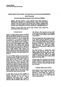
To aid the design of model-predictive controllers, and to assist new users in MPC we have developed a graphical user interface (GUI) for the design and testing of MPC controllers. Fig. 5 shows the interface demonstrating the MIMO control of a 3 degree of freedom model helicopter. The GUI design shows the input/output trends on the left, complete with green/red lights showing if constraints are active. The right panels allow the user to interactively adjust the various horizons, controller weights, and constraints. The tool accepts a wide variety of models: linear discrete or continuous (or a mixture), transfer function or state-space, with, or without deadtime. One can even specify a nonlinear plant, although the model internally used within the MPC will be linearised. The tool also allows one to specify a different dynamic system for the plant than for the model thus enabling the exploration of model/plant mismatches. This is no limit to the size of the models that can be used, but the practicalities of the GUI plotting are such that systems with more than half a dozen i/o rapidly get confusing. However in these cases, one can readily export the data for plotting externally. The screen capture in Fig. 5 also demonstrates the power of MPC. In this case we have a non-square model helicopter plant with 2 input rotors and 3 outputs: azimuth, elevation and pitch. Also depicted are the output constraints (dotted lines), and the future predictions for both the inputs and outputs to the right of the solid line two thirds along the scrolling trend. It is also possible to exchange the system with raw

Figure 5: The Model Predictive Control graphical user interface controlling a 3 DOF Quanser helicopter. Note the depiction of the future input and output predictions. M ATLAB thereby utilising all the existing controller design tools within that environment as well as explicitly constructing the MPC object. For example, for the SIMO plant and model 

   s−1 1.2s − 1.1   ˆ   s+1 1.4s + 1.7 G= ,G =   s+2 1.5s + 2.2 2 2 s + 4s + 5 1.2s + 4.4s + 5.1 (4) with various constraints is coded with 1

% Specify MIMO plant & model Gp=tf({[1,-1],[1 2]}, ... {[1 1],[1 4 5]}); % Plant Gm=tf({[1.2 -1.1],[1.5 2.2]}, ... {[1.4 1.7],[1.2 4.4 5.1]});% Model

6

11

16

3.2

The MPC controller block for Simulink

Fig. 6 shows the MPC controller as implemented in S IMULINK. One needs only to drop our MPC object into the MPC controller block, and, provided the plant is not too dissimilar, the simulation will reproduce a controlled response. Since the S IMULINK tool uses the same MPC object as the GUI described in section 3.1, one could easily export the models and associated properties (constraints, controller horizons etc, and algorithmic details) to the S IMULINK block.

simopts.frm.ydist From simopts.frm.udist Workspace2

Ts=0.1;Np=10;Nc =5; % Ts , Nc , Np setp = 1; % Specify i/o constraints, & controller weights Constraints.u = [-5 5 2.5; -5 5 2.5]; Constraints.y = [-5 5]; Weights.uwt = [0.1 0.2]'; Weights.ywt = [0.1]'; Ex1=jGUI(Gp,Gm,Weights,Constraints, ... Np,Nc,Ts,State_Est,setp);

The MPC object, Ex1 created in the last line of the script can now be directly loaded into the GUI.

y u simopts.frm.setp

u

setp

x delu Discrete Plant ym

yp xm Discrete MPC (sim)

Result

Figure 6: Implementing the MPC controller block for an arbitrary plant in the S IMULINK environment. The jMPC toolbox is available from www.auckland. ac.nz/i2c2.

4

C ONCLUSIONS

The intuitiveness, the ease of tuning, and the optimality are persuasive features of Model Predictive Control which in part account for the increasing interest in industry. However the underlying philosophy of the controller is quite a departure from the classical feedback PID which industry is comfortable with, so to sell the idea of advanced control, we need elegant, easy to use tools. This paper describes one implementation of an MPC controller that is suitable for real-time control, and is the first stage in the development of predictive controllers designed for highspeed embedded applications such as those implemented on FPGA hardware. The maximum obtained sampling frequency for a challenging SISO model is over 1kHz on a 3GHz desktop PC, while sampling rates of 200Hz are possible for the heavily constrained MIMO helicopter case. These numbers, being similar to those reported in [8], suggest that this implementation qualifies for the ‘fast’ MPC label.

ACKNOWLEDGEMENTS Financial support to this project from the Industrial Information and Control Centre, AUT University, New Zealand is gratefully acknowledged.

R EFERENCES [1] C. Garcia, D. Prett, and M. Morari, “Model predictive control: Theory and practice — A survey,” Automatica, vol. 25, no. 3, pp. 335–348, 1989. [2] J. M. Maciejowski, Predictive Control with Constraints. Prentice–Hall, 2002. [3] D. I. Wilson and B. R. Young, “The Seduction of Model Predictive Control,” Electrical & Automation Technology, pp. 27–28, Dec/Jan 2006. ISSN: 1177-2123. [4] S. J. Qin and T. A. Badgwell, “A survey of industrial model predictive control technology,” Control Engineering Practice, vol. 11, pp. 733–764, July 2003. [5] R. Ross, “Revolutionising model-based predictive control,” Computing & Control Engineering Journal, vol. 14, no. 6, pp. 26–29, 2004. [6] L. Wang, Model Predictive Control System Design and Implementation using Matlab. Springer, 2009. [7] J. A. Rossiter, Model-Based Predictive Control: A Practical Approach. CRC Press, 2003. [8] Y. Wang and S. Boyd, “Fast model predictive control using online optimization,” in Proceedings of the IFAC World Congress, (Seoul, Korea), pp. 6974–6997, July 2008.

[9] P. Dua, K. Kouramas, V. Dua, and E. Pistikopoulos, “MPC on a chip — Recent advances on the application of multiparametric model-based control,” Computers & Chemical Engineering, vol. 32, no. 4-5, pp. 754 – 765, 2008. [10] L. G. Bleris, J. Garcia, M. V. Kothare, and M. G. Arnold, “Towards embedded model predictive control for system-on-a-chip applications,” Journal of Process Control, vol. 16, no. 3, pp. 255–264, 2006. Selected Papers from Dycops 7 (2004), Cambridge, Massachusetts. [11] T. A. Johansen, W. Jackson, R. Schreiber, and P. Tøndel, “Hardware synthesis of explicit model predictive controllers,” IEEE Transactions Control Systems Technology, vol. 15, no. 1, pp. 191–197, 2007. [12] G. Valencia-Palomo and J. Rossiter, “Auto-tuned predictive control based on minimal plant information,” in International Symposium on Advanced Control of Chemical Processes ADCHEM 2009, (Istanbul, Turkey), pp. 582–587, International Federation of Automatic Control, 12–15 July 2009. [13] K. Ling, B. Wu, and J. Maciejowski, “Embedded Model Predictive Control (MPC) using a FPGA,” in IFAC Proceedings of the 17th World Congress, (Seoul, South Korea), pp. 15250–15255, 6–11 July 2008. [14] D. E. Seborg, T. F. Edgar, and D. A. Mellichamp, Process Dynamics and Control. Wiley, 2 ed., 2005. [15] E. N. Pistikopoulos, V. Dua, N. A. Bozinis, A. Bemporad, and M. Morari, “On-line optimization via off-line parametric optimization tools,” Computers & Chemical Engineering, vol. 24, no. 2–7, pp. 188–188, 2000. [16] E. N. Pistikopoulos, M. C. Georgiadis, and V. Dua, “Parametric programming & control: from theory to practice,” in 17th European Symposium on Computer Aided Process Engineering (V. Plesu and P. S. Agachi, eds.), vol. 24 of Computer Aided Chemical Engineering, pp. 569–574, Elsevier, 2007. [17] Anon., “Optimization Toolbox User’s Guide,” tech. rep., MathWorks, 3 Apple Hill Drive, Natick, MA, USA, 2009. ˚ [18] J. Akesson, “MPCtools: A toolbox for simulatiuon of MPC controllers in Matlab,” tech. rep., Lund Institute of Technology, Lund, Sweden, January 2006. [19] S. Wright, “Applying new optimization algorithms to model predictive control,” in Fifth International Conference on Chemical Process Control CPC V, pp. 147–155, CACHE Publications, 1997. [20] A. Bemporad, M. Morari, and N. L. Ricker, “Model predictive control toolbox 3,” tech. rep., The Mathworks, 2009.