model selection criterion for sinusoidal signals in Gaussian noise which also contains the log-likelihood and the penalty terms. The simulation results disclose ...
IEEE TRANSACTIONS ON SIGNAL PROCESSING, VOL. 44, NO. I . JULY I996
I744
A Model Selection Rule for Sinusoids in White Gaussian Noise Petar M. DjuriC, Member, IEEE
Abstruct- The model selection problem for sinusoidal signals has often been addressed by employing the Akaike information criterion (AIC) and the minimum description length principle (MDL). The popularity of these criteria partly stems from the intrinsically simple means by which they can be implemented. They can, however, produce misleading results if they are not carefully used. The AIC and MDL have a common form in that they comprise two terms, a data term and a penalty term. The data term quantifies the residuals of the model, and the penalty term reflects the desideratum of parsimony. While the data terms of the AIC and MDL are identical, the penalty terms are different. In most of the literature, the AIC and MDL penalties are, however, both obtained by apportioning an equal weight to each additional unknown parameter, be it phase, amplitude, or frequency. By contrast, in this paper, we demonstrate that the penalties associated with the amplitude and phase parameters should be weighted differently than the penalty attached to the frequencies. Following the Bayesian methodology, we derive a model selection criterion for sinusoidal signals in Gaussian noise which also contains the log-likelihood and the penalty terms. The simulation results disclose remarkable improvement in our selection rule over the commonly used MDL and AIC.
I. INTRODUCTION ODEL SELECTION is an important area of research in signal processing, and its results are applied in many disciplines of science and engineering. Over the past two decades many of these problems have been addressed by utilizing two popular selection rules known as Akaike information criterion, or AIC [ 11, and minimum description length, or MDL [19]-[21]. For example, they have been applied in array processing to detect the number of sources that impinge on a passive sensor array [25], [26] in vibration analysis to decompose a nonstationary vibration record into stationary segments [7], and in image analysis to segment images [12], [ 131. Many more examples can be cited from areas as diverse as econometrics, control theory, and psychometrics The widespread use of these rules is mainly due to their intrinsic simplicity. Neither requires the derivation of test statistics or selection of thresholds from statistical tables-tasks which are both rather difficult, particularly when there are several models to choose from, and/or the examined models are not nested. Instead, the AIC and MDL are simply applied by evaluating two terms, a data term and a penalty term. Manuscript received September 27, 1994; revised January 12, 1996. This work was supported by the National Science Foundation under Award MIP9110628, The associate editor coordinating the review of this paper and approving it for publication was Dr. Monique Fargues. The author is with the Department of Electrical Engineering, State University of New York at Stony Brook, Stony Brook, NY 11794.2350 USA (e-mail: djurice shee.sunysb.edu). Publisher Item Identifier S 1053-587X(96)04525-4.
These two terms are added together, and the model that yields the minimum sum is considered to be the best. In mathematical terms, if the set of competing models is denoted byMI;.kEZQ, whereZ~={O,1,2,...,Q-l},andtheir associated parameters are O k , the model is selected according to [14]
where (81;) is the log-likelihood function of the data, 0 k is the maximum-likelihood (ML) estimate of the parameters O k , and p, is the penalty of the criterion. The difference between the two criteria is in the penalty term p,. The AIC imposes p c = p x ~ c= dI;,and the MDL, p c = ~ M D L= d k / 2 In N / 2 [14]. Here dk: represents the number of parameters associated with the kth model, and N , the length of the observed data vector. These penalties obviously imply that each additional unknown parameter is equally weighted, regardless of its role in the model function. In general, however, it is not appropriate to penalize for additional unknown parameters equally and without regard to their roles in the model. To establish the validity of this claim, we address a specific problem and show that the penalties are parameter dependent. In particular, we investigate a model selection problem where the competing models represent multiple sinusoids in white Gaussian noise. This problem has been of considerable interest since the beginning of the century [ 5 ] , [23],and continues to attract the attention of many researchers [6], [8], [15], [16], [18]. When the selection is implemented by the AIC and MDL, the rules usually employed take the form of [lo], [27], [281 ~ X I C=
arg kmin EZq{-L(Ok)
+3k)
where ~ . A I Cand &,,ID, are the optimal numbers of signal components according to the AIC and MDL, respectively. Note that d k = 3k since each sinusoid is parameterized by its amplitude, phase, and frequency, and that the penalties due to each parameter are identical. Recently, besides (2) and (3), similar selection rules have been proposed. In particular, in [24] a model selection rule for sinusoids in colored noise was proposed whose form is
1053-587)3/96$05 .OO 0 1996 IEEE
Authorized licensed use limited to: SUNY AT STONY BROOK. Downloaded on April 30,2010 at 16:16:03 UTC from IEEE Xplore. Restrictions apply.
DJURIC:SINUSOIDS IN WHITE GAUSSIAN NOISE
174.5
where c is a constant that satisfies c > y,with y depending on the spectral density of the noise process. It was shown that (4) is strongly consistent. However, the use of this criterion is limited because the choice of c depends on the noise spectral density, which is usually unknown. It is important to point out that for white noise y = 2, and c > 2. Noteworthy too are the facts that the results from [24] imply the strong consistency of ( 3 ) , and when c is too small or too large, (4) tends to overestimate or underestimate the number of sinusoids, respectively [9]. For the colored noise problem another criterion was given in [9]. It is indirectly based on the MDL principle but is different from ( 3 ) , and its evaluation is implemented in the frequency domain. There, the main idea is to model the continuous noise spectrum as constant over frequency bands of width 2 r m / N , where N is the number of observed data samples, and m is an integer. The obtained criterion has a penalty that has two terms, one depending on the number of sinusoids k , and the other being a function of m. The best signal model is obtined by optimizing the criterion simultaneously over k and m. For the same problem, one more MDL type criterion was suggested in [11], where the noise is modeled as an autoregression of unknown order. Finally, in [4], a maximum a posteriori probability (MAP) criterion was proposed whose form is
of our model selection criterion in Sections I11 and IV. Various points related to the selection problem are discussed in Section V, and a presentation of simulation results on the performance of the selection rules is given in Section VI. Finally, in Section VI1 some brief conclusions are drawn. 11. PROBLEM STATEMENT Let y be an observed vector of N real data samples. The elements of y may represent samples of noise only,
Yhl
= 4731,
n E 2,
(6)
or m superimposed sinusoids embedded in nois,e, m
y[n] =
aj
cos(wjn
+ 4 j ) + e[nj,
n
E
Znr.
(7)
j=1
Here e[n] symbolizes a noise sample whereas a j ,w j and (ltj are the amplitude, radial frequency, and phase of the jth sinusoid, respectively. Z N is the finite set of integers (0, 1, . . . , N - l}. Without loss of generality, we assume that wj
j
fwl,
w j E(O;7r),
# 1,
j,1 = 1 , 2 , . . . , m
j = 1 , 2 , . ” , m.
(8)
Alternatively, we may represent (7) as m
y[n] =I “ J a j ,
cos(wjn)
+ a j s sin(wjn)) + e[rbl,
nE
zA~
j=l
This criterion is identical to the MDL criteria from [9] and [ 111 when they are also applied to sinusoids in white noise. To make a distinction between the correct and the comrnonly used MDL criteria, we refer to (3) as the “MDL” criterion. A comparison of (5) with (2) and ( 3 ) clearly shows the differences in the penalties and that the penalty in ( 5 ) is the most stringent of the three. In this paper, we derive ( 5 ) and show how the penalties are obtained for additional unknown parameters. In particular, we demonstrate that the penalization per additional unknown amplitude or phase is In N and per addilional unknown frequency In N , which makes a total of j: 1 n N for every additional sinusoid. In using the Bayesian methodology, we apply asymptotic arguments and explain the derivation steps, which can readiily be replicated in obtaining selection rules for other types of models. Aside from the derivation, we discuss important issues of the model selection problem, and we provide extensive simulation results that exhibit the performance of ( 5 ) and compare it to (3). The article is organized as follows. In Section 11the problem statement is given, followed by the definition and derivation
1 cos (w 1)
Dzm =
COS(Wl2)
0 sin(w1) sin(wl2)
-cos(wi(N - 1)) sin(wl(N - I ) )
(9) where ,j = I . 2, . . . , m.
a3, = a3 cos 4 j , a J S = -a3 sin 4J,
Finally, a concise depiction of (9) is provided in a vector-matrix form according to
Y = D2ma27n
+e
(10)
where Dzm is an N x 2m matrix, shown at the bottom of the page, and the amplitude vector ~2~ is given by denoting uTm == [a”, al, azC azS . . . ucm u s m ] ,with transposition. The noise vector is assumed to be zero mean normal with density function
-.,}.
1 2a2
(11)
The number of sinusoids 7n and their parameters are unknown, as is the noise variance 0’. Given y and the aforementioned assumptions, the objective is to determine the number of superimposed sinusoids in y.
... ... ...
1 cos(wm) cos(wm2)
. . . cos(w,(N
0 sin(wm) sin(wm2)
- 1)) sin(w,(N
-
1))-
Authorized licensed use limited to: SUNY AT STONY BROOK. Downloaded on April 30,2010 at 16:16:03 UTC from IEEE Xplore. Restrictions apply.
IEEE TRANSACTIONS ON SIGNAL PROCESSING, VOL. 44, NO. 7, JULY 1996
1146
111. MODELSELECTION CRITERION
OF THE I v . DERIVATION
The formulated problem is clearly one of model selection (multiple hypotheses testing). Based on an accepted criterion, we want to choose the best model for the data from a set of predefined models. As an investigating strategy, the Bayesian methodology and MAP criterion are adopted as they allow for a consistent and optimal solution in a clearly defined way. Let M I , denote the hypothesized model, with k being the number of sinusoids in the data, and let p ( k ) be the a priori probability of the kth model. Formally, when k = 0, the model M Ois represented by (6), and when k > 0,M I , is given by Mk :
y = D2kUzk + e .
(12)
It is assumed that there are Q competing models, where Q > m, and that each model is equiprobable. That is 1
p(k) =
-,
6!
k E ZQ.
f(Ylk) =
(17)
From (6) and ( l l ) , the first factor of the integrand can be expressed as
The second factor, f ( a l k ) ,is the prior density of the standard deviation of the noise which quantifies our initial knowledge of LT. If this knowledge is vague, one typically adopts the Jeffreys' prior [2]
f(a1k) cx a-1
(19)
where cx signifies proportionality. Since we want to derive a model selection criterion that will be based on as little prior knowledge as possible, we adopt (19) as a prior. When (18) and (19) are substituted into (17), and with the use of the integral [2]
U
where
I?(.)
>
0; p
>0
(20)
is the standard Gamma function, it is found that
f(ylk) where f ( y / k ) is the marginalized density of g given there are k sinusoids in the data,' and f ( y ) is the marginal density of the data. Note that under the assumption of (13), the maximization of the a posteriori probability becomes simply a maximization of the marginalized densities o f the models, f ( y 1 k ) . Q and f(y) were dropped from the criterion because they are independent of k . Note that Q is a constant, and
> 0. When
J' f(Y/k,a)f(~lk)da, k = 0.
(13)
The MAP estimate of m will be the value of k that maximizes the a posteriori probability p ( kly). where k E ZQ or
CRITERION
First we derive f(ylk) for k = 0 and then for k k = 0, the form of f ( y l k ) is determined from
r
(3
- ( ~ ~ y ) - ( ~ / ~k )=, 0.
(21)
Now we derive the expression for f ( y ) k )when k > 0 . In order to do so, the following integrals need to be solved:
f ( w k ,ff, a21,lk)d a z k
do dwk,
k
> 0 (22)
where f(wk.a.a21,lk) is the prior of the model parameters. Again, we adopt a vague prior whose form is
I/ f(y/k,a)f(aIk)da,
k =0
(23)
f(Wk,a,a2klk) lx a-1.
The marginalized density f ( y l k ) can be obtained from
First, the innermost integral of (22) is solved yielding f ( y . w k . a l k ) . From (10) and ( l l ) , it is deduced that the first factor of the integrand in (22) is f ( y l k , w I , ,a, U 2 k ) = ( 2 n a 2 ) - ( " 2 ) 1 . exp - s ( y - D z I , ~ z -~DZI,WI,) ) ~ ( ~ . (24)
{
where 5 2 k ; a , and A ~ I ,in (16) represent the parameter spaces of wk,a, and U Z k , respectively, while f ( a l k ) and f(wk,o,aklk) are the a priori densities of a and W I , , ~ and : u ~ I respectively, ,, given the number of sinusoids in the data is k . In the next section we present the derivation of f ( y 1 k ) and provide the final form of the selection criterion. For fixed y, f ( y / k ) can be viewed as the likelihood of k superimposed sinusoids in the data.
1
Applying the prior in (23), one readily obtains
where PkA.is an N x N projection matrix defined by
P $ ~= I
-
D ~ ~ ( D ; ~ D ~ ~ ) - ~ (26) D&.
Authorized licensed use limited to: SUNY AT STONY BROOK. Downloaded on April 30,2010 at 16:16:03 UTC from IEEE Xplore. Restrictions apply.
DJURIC: SINUSOIDS IN WHITE GAUSSIAN NOISE
1141
Next we solve the second integral
From (28), we have
This integral is of the same form as (20). It results in
where C is a constant. Upon taking the first derivative with respect to w;, one obtains
T
I
. ( Y P,,Y)
-((N-25)/2)
(37)
Finally, we want to integrate out the frequencies
f ( Y l k ) = /ak
wk,
f(Y,Wklk)
i.e., find (29)
As the frequencies are nonlinear parameters, it is very difficult to obtain an analytical solution, and we thus resort to approximations. If f ( y , w k l k ) is Taylor expanded around the ML estimate of wk, one can write
where the derivative with respect to the determinant ID; D 2 k I has been neglected since the determinant is almost constant over f l k when the conditions specified in (8) hold. Now, after taking the partial derivative of (37') with rcspect to w I , we find a2 _____
ln f (Y, W k I k ) aW,aW3
f ( Y , W / t l k ) = exP{ln.f(Y,wkIk)} N exp{ln f(yI&, k )
N
N
- Z1 ( W ~- c & ) ~ Q ~ (-w&)} ~
-
2k
-___
-
(30)
2
N - 2k where Gk is the ML estimated of wk, and f7k is the Hessian of -Inf(y,wkIk) evaluated at wk = Gk,or
(Y 1% Y 1(38)
With (34) and (35) it can be shown that If (30) is substituted in (29). the integration becomes straightforward. The result can be expressed as f ( y / l k ) cx f(y1Gjrc. k ) l Q k l - ( ~ / 2 ) .
G k =
N3Rk
(33)
where R k is a k x k positive definite matrix whose determinant is of order O(1). The proof is not difficult but rather tedious. The following results will be used as we proceed [22]:
1 ~
N,++1 1
3%
(32)
We would like to simplify (32) so that the evaluation of the Hessian may be avoided. To this end, we apply the following proposition. Proposition: When N is large, the Hessian of -In f ( y , wklk) can be written as
T
-Y
I
P,kY =O(N)
(39)
dW,dWJ Y P 2 , Y =
T
I
(40)
T
I
(41)
Y P,kY =O(N).
If the results (39)-(41) are applied to (38), the claim in the proposition directly follows. Returning to (32) and using the main result of the proposition as well as (28), we can express the marginal dmsity f ( Y I k ) by
N - 2k
. ( y ~ ~ ~ k y ) - ( ( ~ - 2 k ) / 2 ) ~ - ( 3 k i I2k,kl-(1/2) ) (42)
N-l
nk cos(wn) rv 0
-1
n=O N-l
nk sin(wn)
p?
0.
(34)
n=O
where D , k and P,, are the matrices D,, and Pik,respectively, with wk substituted by Gk.With this result, the final form of the model selection criterion can readily be established as
In addition, if A is a matrix whose entries are functions of w k , one can write [17]
riZMAp
= arg min { - In f(ylk)} kCzQ
(43)
(35)
Authorized licensed use limited to: SUNY AT STONY BROOK. Downloaded on April 30,2010 at 16:16:03 UTC from IEEE Xplore. Restrictions apply.
IEEE TRANSACTIONS ON SIGNAL PROCESSING, VOL. 44, NO.
1748
(44) where in the last expression we have dropped all the terms of order 0(1),and we have assumed that N is large. We further simplify (44) by observing that IP;kD2kI
YTPikY
=0(NZk)
(45)
=O ( N )
(46)
and that the relative contribution of the Gamma function in (44) can asymptotically be replaced by k l n N . To understand the latter approximation, divide - In f(ylk) in (44) by I ' ( N / 2 ) .This does not change the criterion because r'(N/2) is not a function of k , and the resulting penalty readily follows. With these approximations, one can obtain the final form of the criterion as
V. DISCUSSION In this section we go on with discussion of several important issues related to (47). 0 First we provide an interpretation of the result in (47). Note that the AIC and "MDL" rules in (2) and (3) can be written as ~?L.AJC=
arg min
kEZQ
{
I In(yTP,,y)
+3k}
(48)
fi>hMDL) = arg min which allow for a direct comparison with (47). Needless to say, the MAP criterion imposes a stricter penalty than either the AIC or MDL. Even more interesting is the fact that the MAP rule penalizes for the extra parameters with penalties that depend on the type of parameters used in the models, which is in contrast to the AIC and MDL. In particular, from our derivation, it is easy to deduce that the penalization for each amplitude or phase is In N , and for each frequency $ In N . The different penalties can be interpreted as follows. Suppose that the MAP criterion can be approximated as the minimizer of - ln(f(yI81;, 6,k ) f ( O k ) ) over k , where 81;and 6 denote the ML estimates of the signal parameters and the noise variance, respectively, and f(81;)is the prior of the signal parameters which is chosen to be a constant that depends somehow on 81;.Suppose also that the ML estimates of the signal parameters are obtained by a grid search. Once we decide about the grid size, the prior of the signal parameters is selected to be uniform over the grid. An open and sensitive question is how to choose the grid size. A reasonable choice is to adopt a grid which is a function of the data record length N , or more precisely, a function of the estimation accuracy with which 8, are obtained. Now, recall that the Cramer-Rao bound of the sinusoidal parameters is proportional to 1/N for the amplitudes and phases and l / N 3 for the frequences. Then,
I, JULY 1996
if the priors of the unknown signal parameters are chosen as proposed, i.e., for each amplitude and phase they are equal to 1/N and for each frequency l/N3, the criterion function in (47) follows immediately from - ln(f(yl81;; 6 ,k ) f ( 8 , ) ) . 0 The result in (47) can also be obtained by a different derivation. If we expand the density f ( y , ~ k , o , a 2 1 ; l k )in a Taylor expansion around the ML estimates of the parameters, ignore the prior due to the asymptotic assumptions, and approximate the determinant of the Hessian by neglecting all the terms that are not a function of N , we obtain the same rule as (47). 0 It can be shown that a similar rule holds for complex sinusoids. In [3] we have investigated this problem by exploiting the concept of predictive densities which is yet another way to find (47). To obtain the rule for complex data that is equivalent to (47), upon deriving the final results in [3], one has to make an additional step which includes asymptotical approximations. 0 It may be tempting to use an algorithm which would avoid the evaluation of the criterion function for every model [24]. In particular, we might want to rely on the following phenomenon: As the model complexity increases, the criterion function decreases until it reaches the minimum at the correct model, and then increases as the models becomes more complex. In other words, if the criterion function is
than we might propose to choose the best model according to m = min{k:
J1;5 J ~ + I }
k EQ
The last expression is attractive because we start with evaluating the criterion function of the simplest (noise) model and then escalate the complexity of the models by sequentially adding one more sinusoid until the criterion functions of J1; and J,+l meet the condition J1; 5 J k + l . Obviously, by implementing the MAP rule with this strategy, we avoid the examination of all the models. This is, however, not recommended because we cannot guarantee that the first minimum of the criterion function is achieved at the correct model. To show this, consider the following experiment. Let y be of fixed length N with a fixed noise sequence e. If y contains sinusoids, using (51), we will incorrectly choose the noise model M O if
Suppose that for some m (52) is not satisfied. Now, we start adding new sinusoids to the data, which will imply a steady decrease of the term on the left side of (52). After a sufficient number of sinusoids has been added, the value of the logarithm on the left side of the inequality will drop below y,and we will choose the noise only model. This will happen when the data actually contain many sinusoids, thus incurring a gross error in
Authorized licensed use limited to: SUNY AT STONY BROOK. Downloaded on April 30,2010 at 16:16:03 UTC from IEEE Xplore. Restrictions apply.
DJURIC. SINUSOIDS IN WHITE GAUSSIAN NOISE
1749
C -4 0
3 4 aJ
% 4
d 2 U aJ 0 U
U 0 U4
0
a U 0
a U In
w
C
0
-4 Y
2 -4
c, In
aJ
4
e,
m C
w 0
a 0 a U m
W
1 C
0 -4 U
2
0.8
-4 c In , Q)
0.6
aJ
0 > U-
0
-=:
0.4
a 0.2 c,
w In
-2
0
2
4 (c) SNR[dBI
6
10
(C)
Fig. I. (a) Estimated probabilities of correct selection. (b) Model underestimation. (c) Model overestimation. The solid and the dashed lines represent the MAP and the MDL performances, respectively.
the selection. In conclusion, one should not apply (51) when k is increasing If we apply a modified rule by starting with the most complex model with k steadily decreasing, there still exists the possibility of a local minimum occurring before we reach the global minimum, and that may be a consequence of
noise modeling. Thus the use of (51) or an equivalent rule is not encouraged. 0 F'inally, the results of (47) depend critically on the quality of the ML estimates. We found that if an iterative algorithm is employed for parameter estimation, the final results can
Authorized licensed use limited to: SUNY AT STONY BROOK. Downloaded on April 30,2010 at 16:16:03 UTC from IEEE Xplore. Restrictions apply.
1750
IEEE TRANSACTIONS ON SIGNAL PROCESSING, VOL. 44, NO. 7, JULY 1996
TABLE I1 MAPAND MDL CRITERIA FOR VARIOUS DATA RECORDLENGTHS FOREACHl v THERE WERE 100 TRIALS. THEENTRIES REPRESEYT THE NUMBER OF TIMES A PARTICULAR MODELWAS SELECTED OUT OF PERFORMANCE COMPARISON OF
100 TRIALS. THECORRECT MODELIS
k=O ‘MDL’ - 3 d B MAP ‘MDL’ - 2 d B MAP ‘MDL’ - l d B MAP ‘MDL’ OdB MAP ‘MDL’ 1 d B MAP ‘MDL’ 2 d B MAP ‘MDL’ 3dB MAP ‘MDL’ 4 d B MAP ‘MDL’ 5 d B MAP
0
k=l 3 28
0
0
0
0 0 0
9 0 3 0 0 0 0
0 0 0
0 0 0
0
0 0
0
0 0 0
k=2 63 70 64 88 72
k=3 23 2 20 3 17
k=4
k=5
6 0
5 0 7
N=72
0 6
0
N=80
9
N=64
5
96
1
0
10
6
0 3
N=88
81
99 73 98 73 99 77 100 66 100 74 99
1
0
0
N=96
15
S
2
0 8
4 0 4
15 1
16 0 19 0
.
N=128
k=O ‘MDL’ 0 MAP 0 ‘MDL’ 0 0 MAP ‘MDL’ 0 0 MAP 0 ‘MDL’ 0 MAP 0 ‘MDL’ 0 MAP ‘MDL’ 0 0 MAP
COMPRISED OF
k=l 0 0 0 0
k=2 0 0 0
0
0
0
0
0 0 0
0 0 0 0
0 0
0 0 0
0
THREE SINUSOIDS ( k = 3 )
k=3 k=4 63 21 95 5 69 17 100 0 70 16 1 0 0 0 68 25 100 0 74 19 99 1 80 18 100
0
k=5 16 0
14 0
14 0 7 0 7 0 2 0
0
0 3
4 0 7
always overestimated the model, most of the time choosing the most complex model which represented five sinusoids 0 0 in noise, and, therefore, we did not include its results in 17 3 6 0 the figures. The MAP rule had an excellent performance for 1 0 0 0 SNR’s above -1 dB, whereas the MDL was always yielding correct results ranging between 59 and 75 times out of 100. strongly depend on the selected convergence criterion. For The deterioration in performance below -1 dB for the MAP example, if convergence in the estimates is declared prema- estimator is not surprising because the ML estimator does turely, despite some moderate differences in their values from not provide good estimates of the frequencies in that range. one iteration to another, poor selections can be obtained. The performance of the MDL starts to deteriorate similarly for slightly lower SNR’s. Again, the results in that range are VI. SIMULATION RESULTS questionable because the frequency estimates are not reliable. In the second experiment we kept all the parameters from In this section we present experimental results that demonstrate the performance of the selection rules. Three experi- the first experiment the same except that we changed the The SNR ments were considered. In the first, the data were generated amplitude of the second sinusoid to a2 = was again varied, this time between 5 dB and -3 dB (for the according to second sinusoid, or equivalently between 10 and 2 dB for the y[n] = a1 cos(w1n $1) U2 cos(wz1z 42) first sinusoid). The results are given in Table I. Practically, e[n], n E ZN ( 5 3 ) identical performance was obtained as in the first experiment. Finally, in the third experiment the data represented three where closely spaced sinusoids. The data y were generated by a1 = a2 = q ! ~=~ 0 rad, $2 = ?r/4 rad. 0 0 0 0
0
S 0
J6.3246.
+
+
+
+
and N = 64. Throughout the experiment, the SNR defined by
where
d%,
(54)
a1
= a3 =
was varied from -3 to 10 dB in steps of 1 dB. The noise sequences were generated according to a Gaussian density function given by (11) with cr2 appropriately chosen to yield the required SNR. For each SNR, there were 100 trials. The maximum number of sinusoids was assumed to be 5. Consequently, the selection rules had to choose the best model out of six nested models. The method for the frequency ML estimation was the one from [22]. The initial estimates were obtained by employing periodograms and notched periodograms [lo]. The results of the simulations for the MAP and the MDL rules are shown in Fig. 1. In Fig. l(a), we present the curves of correct model selection, and in Fig. l(b) and l(c), the curves of overestimation and underestimation, respectively. The AIC
42
= ~ / 4rad,
a2 $3
=
d m ,
= 0 rad,
= ~ / 3 , w1 = 27r 0.2,
The SNR for the first and third sinusoids was 10 dB (and for the second 5 dB). The number of samples was varied and in the first 100 trials it was 64. Then it was increased to 72, 80, 88,96, and 128, and for each data length, there were 100 trials. The results are shown in Table 11. Again, the MAP rule had excellent performance. The results of the MDL were similar as in the previous experiment showing a large percentage of overestimated models. However, as the number of samples was doubled from 64 to 128, its performance improved.
Authorized licensed use limited to: SUNY AT STONY BROOK. Downloaded on April 30,2010 at 16:16:03 UTC from IEEE Xplore. Restrictions apply.
DJURIC: SINUSOIDS IN WHITE GAUSSIAN NOISE
VII. CONCLUSION In this paper, we proposed a model selection rule for sinusoids in Gaussian noise based on the MAP criterion. The rule has a log-likelihood and penalty terms, just like the AIC and MDL. The MAP criterion is different from the other two in the penalty term which is equal to 5 k / 2 In N , where k is the number of sinusoids and N the length of the observed data. The deriv