ISSN 1749-3889 (print), 1749-3897 (online) International Journal of Nonlinear Science Vol.13(2012) No.3,pp.308-316
A Modified Homotopy Perturbation Method for Solving Linear and Nonlinear Integral Equations N. Aghazadeh∗ , S. Mohammadi Department of Applied Mathematics, Azarbaijan University of Tarbiat Moallem, Tabriz 53751 71379, Iran (Received 23 June 2011 , accepted 15 January 2012)
Abstract: In this paper, we present a modification to so-called homotopy perturbation method for solving linear and non-linear integral equations. This method gives an approximate analytic solution to the equations (usually the exact solution of the equations). Some numerical examples presented to show the accuracy and efficiency of the method. Keywords: homotopy perturbation method; integral equation; Fredholm; Volterra
1
Introduction
Although perturbation techniques are widely applied to analyze nonlinear problems in science and engineering, they are however so strongly dependent on small parameters appeared in equations under consideration that they are restricted only to weakly nonlinear problems. For strongly nonlinear problems which don’t contain any small parameters, perturbation techniques are invalid. So, it seems necessary and worthwhile developing at new kind of analytic technique independent of small parameters. Liao proposed a new analytic technique in his Ph.D. dissertation [1], namely the Homotopy Analysis Method (HAM). Based on homotopy of topology, the validity of the HAM is independent of whether or not there exist small parameters in considered equations. Therefore, the HAM can overcome the foregoing restrictions and limitations of perturbation techniques so that it provides us with a powerful tool to analyze strongly nonlinear problems. [2] In [2] some basic ideas about the HAM was described. In [3] some developments of the HAM was presented. Also some lemmas and theorems was proved. In [4] a reliable approach for convergence of the HAM was discussed. In [10]– [14] [46]–[48] [51]–[53] the HAM was applied on some equations. Also, some modifications and improvements was discussed by authors (e.g. see [15]–[17]). In [19, 20] the homotopy perturbation technique was presented. In [21]–[41] [49]–[50][54]–[55] the homotopy perturbation technique was applied on different equations by some authors and with some modifications (e.g. linear and nonlinear forth-order boundary value problems, functional integral equations, nonlinear problems, system of nonlinear Fredholm integral equations, forth-order integro-differential equations, eighth-order boundary value problems, nonlinear oscillators, partial differential equations, quadratic Riccati differential equation, Volterra integral equations, two-dimensional Fredholm integral equations, Stokes equations and nonlinear ill-posed operator equations). Also the homotopy perturbation method and the HAM was compared by some authors (e.g. [5]–[9]). We now review [39] to show how HPM applied to the following integral equations. Consider the following integral equation: ∫ b γ(x) = f (x) + k(x, t)γ(t)dt, c 6 x 6 d. (1) a
Let
∫
b
L(u) = u(x) − f (x) −
k(x, t)u(t)dt = 0, a
∗ Corresponding
author.
E-mail address:
[email protected] c Copyright⃝World Academic Press, World Academic Union IJNS.2012.06.15/610
(2)
N. Aghazadeh, S. Mohammadi: A Modified Homotopy Perturbation Method for Solving Linear and Nonlinear Integral Equations 309
with solution u(x) = γ(x), we can define a homotopy H(u, p) by H(u, 0) = F (u), H(u, 1) = L(u),
(3)
where F (u) is a functional operator with solution u0 .We choose a convex homotopy H(u, p) = (1 − p)F (u) + pL(u) = 0,
(4)
and continuously trace an implicitly defined curve from a starting point H(u0 ) to a solution H(γ, 1). In fact HPM uses the homotopy parameter p as an expanding parameter [43, 44] to obtain u = u0 + pu1 + p2 u2 + · · · ,
(5)
when p → 1, (5) corresponds to (4) and gives an approximation to the solution of (2) as: γ = lim u = u0 + u1 + u2 + · · · , p→1
(6)
The series (6) converges in most cases, and the rate of convergence depends on L(u). Taking F (u) = u(x) − f (x), and substituting (5) in (4) and equating the terms with identical power of p, we obtain u0 − f (x) = 0 ⇒ u0 = f (x), ∫ b u1 − k(x, t)u0 (t)dt = 0,
p0 : p1 :
a
∫
b
u1 =
k(x, t)u0 (t)dt, a
.. . and in general we have u0 (x) = f (x), ∫ b un+1 (x) = k(x, t)un (t)dt,
(7) n = 1, 2, . . . .
(8)
a
2
The new modified HPM
In [39] modification applied to HPM for linear integral equations with degenerate kernels, which used a number m. In this paper, m is a function (or a number), and our modification can be applied to linear or non-linear integral equations, and there is no limitation on kernel type.
2.1
Application to linear second kind Fredholm integral equation
In this section, we apply the modified perturbation method to (1). To this end, we define a new convex homotopy perturbation as H(u, p, m) = (1 − p)F (u) + pL(u) + p(1 − p)mK ∗ f = 0, (9) ∫b ∫ b where F (u) = u(x) − f (x), L(u) = u(x) − f (x) − a k(x, t)u(t)dt = 0 and K ∗ f = a k(x, t)f (t)dt, hence we can write [ ] ∫ b (1 − p)(u − f ) + p u − f − k(x, t)u(t)dt + p(1 − p)mK ∗ f = 0, (10) a
or
∫
b
u−f −p
k(x, t)u(t)dt + p(1 − p)mK ∗ f = 0,
a
IJNS homepage: http://www.nonlinearscience.org.uk/
(11)
310
International Journal of Nonlinear Science, Vol.13(2012), No.3, pp. 308-316
Substituting (5) into (11) and equating the coefficients of like terms with the identical powers of p , we obtain
p1 :
u0 − f (x) = 0 ⇒ u0 = f (x), ∫ b u1 − k(x, t)u0 (t)dt + mK ∗ f = 0,
p2 :
u1 = (1 − m)K ∗ f, ∫ b u2 − k(x, t)u1 (t)dt − mK ∗ f = 0,
p3 :
u2 = (1 − m)K ∗ K ∗ f + mK ∗ f, ∫ b u3 − k(x, t)u2 (t)dt = 0,
p0 :
a
a
a
∫
b
u3 =
k(x, t)u2 (t)dt, a
.. .
∫
pn+1 :
b
un+1 =
k(x, t)un (t)dt,
n = 2, 3, . . . ,
a
now we find m such that u2 = 0. Since if u2 = 0 then u3 = u4 = · · · = 0, and the exact solution will be obtained as u(x) = u0 (x) + u1 (x), hence for all values of x we should have (1 − m)K ∗ K ∗ f + mK ∗ f = 0, or m(x) =
K ∗K ∗f · − K ∗f
K ∗K ∗f
Note that the method can be applied as for Volterra integral equations, in same manner.
2.2
Application to non-linear Fredholm integral equations
Consider the following non-linear Fredholm integral equation ∫
b
k(x, t)T (u(t))dt, a 6 x 6 b
u(x) = f (x) +
(12)
a
where the function k is given and T is a given nonlinear operator, and u the solution to be determined. We assume that (12) has the unique solution. We define a convex homotopy perturbation as H(u, p, m) = (1 − p)F (u) + pL(u) + p(1 − p)mK ∗ T (f ) = 0, where
∫ F (u) = u(x) − f (x) and L(u) = u(x) − f (x) −
(13)
b
k(x, t)T (u(t))dt = 0,
(14)
a
hence, we can write [
∫
b
(1 − p)(u − f ) + p u − f −
] k(x, t)u(t)dt + p(1 − p)mK ∗ T (f ) = 0,
(15)
a
or
∫
b
u−f −p
k(x, t)u(t)dt + p(1 − p)mK ∗ T (f ) = 0,
(16)
a
Substituting (5) into (16) results into ∫
b
u0 + pu1 + p2 u2 + · · · − f (x) − p
k(x, t)T (u0 + pu1 + p2 u2 + · · · )dt + p(1 − p)mK ∗ T (f ) = 0
a
IJNS email for contribution:
[email protected]
(17)
N. Aghazadeh, S. Mohammadi: A Modified Homotopy Perturbation Method for Solving Linear and Nonlinear Integral Equations 311
In (17) we can write T (u0 + pu1 + p2 u2 + · · · ) as follows T (u0 + pu1 + p2 u2 + · · · ) = A0 + pA1 + p2 A2 + · · · ,
(18)
where Ak are Adomian polynomials which depend upon u0 , u1 , u2 , . . . , uk . [39, 45] By differentiating both sides of (18) we can write dk dk 2 T (u + pu + p u + · · · ) | = (A0 + pA1 + p2 A2 + · · · ) |p=0 . (19) 0 1 2 p=0 dpk dpk From (19) we have 1 dk T (u0 + pu1 + p2 u2 + · · · ) |p=0 , k! dpk
Ak = Ak (u0 , u1 , u2 , . . . , uk ) =
k = 0, 1, . . .
(20)
By substituting (18) into (17) we have ∫
b
u0 + pu1 + p2 u2 + · · · − f (x) − p
k(x, t)(A0 + pA1 + p2 A2 + · · · )dt + p(1 − p)mK ∗ T (f ) = 0.
(21)
a
Equating the terms with identical powers of p, we have
p1 :
u0 − f (x) = 0 ⇒ u0 = f (x), ∫ b u1 − k(x, t)A0 (t)dt + mK ∗ T (f ) = 0,
p2 :
u1 = (1 − m)K ∗ T (f ), ∫ b u2 − k(x, t)A1 (t)dt − mK ∗ T (f ) = 0,
p3 :
u2 = K ∗ ((1 − m)K ∗ T (f )T ′ (f )) + mK ∗ T (f ), ∫ b u3 − k(x, t)A2 (t)dt = 0,
p0 :
a
a
a
∫ u3 =
b
k(x, t)A2 (t)dt, a
.. .
∫
pn+1 :
un+1 =
b
k(x, t)An (t)dt,
n = 3, 4 . . . ,
a
now we find m such that u2 = 0. Since if u2 = 0 then u3 = u4 = · · · = 0, and the exact solution will be obtained as u(x) = u0 (x) + u1 (x), hence for all values of x we should have (1 − m)K ∗ (K ∗ T (f )T ′ (f )) + mK ∗ T (f ) = 0, or
K ∗ (K ∗ T (f )T ′ (f )) · K ∗ (K ∗ T (f )T ′ (f )) − K ∗ T (f ) Note that the method can be applied as for Volterra integral equations, in same manner. m(x) =
3
Numerical Examples
Example 1 Consider the equation
∫
π
u(x) = (1 − 2π) cos x + sin x +
4 cos x cos tu(t)dt, 0
with exact solution u(x) = sin x + cos x. Using the method, we have u0 = f (x), u1 = (1 − m)K ∗ f, where
m(x) =
K ∗K ∗f K ∗K ∗f − K ∗f
IJNS homepage: http://www.nonlinearscience.org.uk/
(22)
312
International Journal of Nonlinear Science, Vol.13(2012), No.3, pp. 308-316
and K ∗f =
∫
b
k(x, t)f (t)dt a
u(x) = u0 + u1 . In this example K ∗ f = 2(1 − 2π)π cos x and K ∗ K ∗ f = 4(1 − 2π)π 2 cos x hence 2π , −1 + 2π u0 = (1 − 2π) cos x + sin x, u1 = 2π cos x
m(x) =
so we have u(x) = cos x + sin x, which is the exact solution. Example 2 Consider the following Fredholm integral equation 1
u(x) = e2x+ 3 −
1 3
∫
1
5
e2x+ 3 t u(t)dt, 0
with exact solution u(x) = e2x . 1 1 1 1 In this example K ∗ f = −(−1 + e 3 )e 3 +2x and K ∗ K ∗ f = (−1 + e 3 )2 e 3 +2x hence m(x) = 1 −
1 1
e3
1
u0 = e2x+ 3 , 1 u1 = −(−1 + e 3 )e2x so we have u(x) = e2x , which is the exact solution. Example 3 Consider the following Volterra integral equation x6 u(x) = 12x + x − 2x − − 11 sin x + 2 30 2
∫
x
(x − t)3 u(t)dt,
3
0
with exact solution u(x) = x2 + sin x. In this example (
) 3x5 x6 x7 x10 K f = 2 66x − 11x + + − − − 66 sin x 5 60 70 25200 ∗
3
and K ∗ K ∗ f = 1584x − 264x3 +
66x5 11x7 x9 x10 x11 x14 − + + − − − 1584 sin x 5 35 210 12600 23100 25225200
hence m(x) = x(−39956716800 + 6659452800x2 − 332972640x4 + 7927920x6 − 120120x8 − 2002x9 + 1092x10 + x13 ) + 39956716800 sin x x(−36626990400 + 6104498400x2 − 302702400x4 + 840840x5 + 7207200x6 − 120120x8 − 4004x9 + 1092x10 + x13 ) + 36626990400 sin x x6 2 3 u0 = 12x + x − 2x − − 11 sin x, 30 u1 = 143(x(−1663200 + 277200x2 − 15120x4 − 420x5 + 360x6 + x9 ) + 1663200 sin x)2 900(x(−36626990400 + 6104498400x2 − 302702400x4 + 840840x5 + 7207200x6 − 120120x8 − 4004x9 + 1092x10 + x13 ) + 36626990400 sin x) u(x) = 12x + x
2
x6 3 − 2x − − 11 sin x + 30 143(x(−1663200 + 277200x2 − 15120x4 − 420x5 + 360x6 + x9 ) + 1663200 sin x)2
900(x(−36626990400 + 6104498400x2 − 302702400x4 + 840840x5 + 7207200x6 − 120120x8 − 4004x9 + 1092x10 + x13 ) + 36626990400 sin x)
IJNS email for contribution:
[email protected]
N. Aghazadeh, S. Mohammadi: A Modified Homotopy Perturbation Method for Solving Linear and Nonlinear Integral Equations 313
Example 4 Consider the following Volterra integral equation ∫ x u(x) = x − sinh(x − t)u(t)dt, 0 3
with exact solution u(x) = x − x6 . Here, K ∗ f = x − sinh x and K ∗ K ∗ f = x + 12 x cosh x − m(x) =
3 sinh x 2
hence
2x + x cosh x − 3 sinh x x cosh x − sinh x
u0 = x, u1 = − u(x) =
2(x − sinh x)2 x cosh x − sinh x
−2x2 + x2 cosh x + 3x sinh x − 2 sinh x2 x cosh x − sinh x
Example 5 Consider the following Volterra integral equation u(x) =
1 (7 cos x + 9 cos 3x + 4x sin x) − 16
∫
x
(x − t) cos(x − t)u(t)dt, 0
with exact solution u(x)( = 13 (2 cos 3x + 1). ) 1 Here, K ∗ f = 1536 −3(45 + 56x2 ) cos x + 135 cos 3x − 4x(15 + 8x2 ) sin x and K ∗K ∗f =
( ) 1 5(−675 + 24x2 + 224x4 ) cos x + 3375 cos 3x + 4x(3345 + 40x2 + 32x4 ) sin x 245760
hence m(x) =
5(−675 + 24x2 + 224x4 ) cos x + 3375 cos 3x + 4x(3345 + 40x2 + 32x4 ) sin x 5(3645 + 5400x2 + 224x4 ) cos x − 18225 cos 3x + 4x(5745 + 1320x2 + 32x4 ) sin x
1 (7 cos x + 9 cos 3x + 4x sin x), 16 5(3(45 + 56x2 ) cos x − 135 cos 3x + 4x(15 + 8x2 ) sin x)2 u1 = − 48(5(3645 + 5400x2 + 224x4 ) cos x − 18225 cos 3x + 4x(5745 + 1320x2 + 32x4 ) sin x)
u0 =
u(x) =
1 1536
( 96(7 cos x + 9 cos 3x + 4x sin x) −
( )2 160 3(45 + 56x2 ) cos x − 135 cos 3x + 4x(15 + 8x2 ) sin x
)
5(3645 + 5400x2 + 224x4 ) cos x − 18225 cos 3x + 4x(5745 + 1320x2 + 32x4 ) sin x
Example 6 Consider the following nonlinear Volterra integral equation ∫ x 2 u(x) = 1 + sin x − 3 sin(x − t)u2 (t)dt, 0
with exact solution u(x) = cos x. Using the method, we have u0 = f (x), u1 = (1 − m)K ∗ T (f ),
where
m(x) =
K ∗ (K ∗ T (f )T ′ (f )) − K ∗ T (f )
K ∗ (K ∗ T (f )T ′ (f ))
and K ∗ T (f ) =
∫
b
k(x, t)T (f (t))dt a
u(x) = u0 + u1 . In this problem K ∗ T (f ) = K ∗ (K ∗ T (f )T ′ (f )) =
1 40
(−285 + 344 cos x − 60 cos 2x + cos 4x) and
1 (−176509 cos x + 7315 cos 2x − 3(−57750 + 1505 cos 3x − 154 cos 4x + cos 6x + 30100x sin x)) 5600
IJNS homepage: http://www.nonlinearscience.org.uk/
314
International Journal of Nonlinear Science, Vol.13(2012), No.3, pp. 308-316
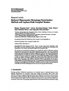
Table 1: The values of absolute error for examples 3–6. x example 3 example 4 example 5 example 6 0.1 1.40e-14 2.183e-11 2.082e-9 5.735e-10 0.2 2.15e-14 2.790e-9 1.329e-7 1.42e-7 0.3 2.78e-13 4.759e-8 1.509e-6 3.423e-6 3.556e-7 8.435e-6 3.148e-5 0.4 8.85e-12 1.691e-6 3.196e-5 1.689e-4 0.5 1.63e-10 0.6 1.76e-9 6.036e-6 9.464e-5 6.397e-4 0.7 1.32e-8 1.768e-5 2.363e-4 1.895e-3 0.8 7.54e-8 4.480e-5 5.202e-4 4.668e-3 0.9 3.52e-7 1.016e-4 1.040e-3 9.964e-3 1.0 1.40e-6 2.111e-4 1.927e-3 1.896e-2 hence m(x) =
176509 cos x − 7315 cos 2x + 3(−57750 + 1505 cos 3x − 154 cos 4x + cos 6x + 30100x sin x) , −193200 + 200589 cos x − 11515 cos 2x + 4515 cos 3x − 392 cos 4x + 3 cos 6x + 90300x sin x
u0 = 1 + sin2 x, u1 =
7(−285 + 344 cos x − 60 cos 2x + cos 4x)2 , 4(−193200 + 200589 cos x − 11515 cos 2x + 4515 cos 3x − 392 cos 4x + 3 cos 6x + 90300x sin x)
u(x) = 1 + sin x2 +
7(−285 + 344 cos x − 60 cos 2x + cos 4x)2 . 4(−193200 + 200589 cos x − 11515 cos 2x + 4515 cos 3x − 392 cos 4x + 3 cos 6x + 90300x sin x)
References [1] S.J. Liao, The homotopy analysis method and its applications in mechanics, Ph.D. thesis, Shanghai Jiaotong University. 1992. [2] S.J. Liao, Homotopy analysis method: a new analytic method for nonlinear problems, Applied Mathematics and Mechanics, 19(10)(1998):957–962. [3] S.J. Liao, Notes on the homotopy analysis method: Some definitions and theorems, Commun Nonlinear Sci Numer Simulat, 14(2009):983–997. [4] Z.M. Odibat, A study on the convergence of homotopy analysis method, Applied Mathematics and Computation, 217(2010):782–789. [5] S. Liang and D. Jeffrey, Comparison of homotopy analysis method and homotopy perturbation method through an evolution equation, Commun Nonlinear Sci Numer Simulat, 14(2009):4057–4064. [6] M.S.H. Chowdhury, I. Hashim and O. Abdulaziz, Comparison of homotopy analysis method and homotopy perturbation method for purely nonlinear fin-type problems, Commun Nonlinear Sci and Numer Simulat, 14(2009):371–378. [7] M. Sajid and T. Hayat, Comparison of HAM and HPM methods in nonlinear heat conduction and convection equations, Nonlinear Analysis: Real World Applications, 9(2008):2296-2301. [8] S. Liao, Comparison between the homotopy analysis method and homotopy perturbation method, Applied Mathematics and Computation, 169(2005):1186–1194. [9] S. Liang and D.J. Jeffrey,Comparison of homotopy analysis method and homotopy perturbation method through an evolution equation, Commun Nonlinear Sci Numer Simulat, 14(2009):4057-4064. [10] Z. Niu and C. Wang, A one-step optimal homotopy analysis method for nonlinear differential equations, Commun Nonlinear Sci Numer Simulat, 15(2010):2026–2036. [11] S.J. Liao, An optimal homotopy analysis approach for strongly nonlinear differential equations, Commun Nonlinear Sci Numer Simulat, 15(2010):2003–2016. [12] H. Jafari and M.A. Firoozjaee, Multistage homotopy analysis method for solving nonlinear integral equations, Applications and Applied Mathematics: An International Journal, Special Issue (1)(2010):34–45. [13] Y.H. Qian, W. Zhang , B.W. Lin and S.K. Lai, Analytical approximate periodic solutions for two-of-freedom coupled van der pol-Duffing oscillators by extended homotopy analysis method, Acta Mech, DOI 10.1007/s00707-010-04333.
IJNS email for contribution:
[email protected]
N. Aghazadeh, S. Mohammadi: A Modified Homotopy Perturbation Method for Solving Linear and Nonlinear Integral Equations 315
[14] A.S. Bataineh, M.S.M. Noorani and I. Hashim, Solving systems of ODEs by homotopy analysis method, Commun Nonlinear Sci Numer Simulat, 13(2008):2060–2070. [15] S.S. Motsa, P. Sibanda, G.T. Marewo and S. Shateyi, A note on improved homotopy analysis method for solving the Jeffery-Hamel flow, Mathematical Problems in Engineering, Volume 2010, Article ID 359297, 11 pages. [16] A.S. Bataineh, M.S.M. Noorani and I. Hashim, Modified homotopy analysis method for solving systems of secondorder BVPs, Commun in Nonlinear Scie and Numer Simulat, 14(2009):430–442. [17] R.A. Van Gorder and K. Vajravelu, On the selection of auxiliary functions, operators, and convergence control parameters in the application of the homotopy analysis method to nonlinear differential equations: a general approach, Commun Nonlinear Sci Numer Simulat, 14(2009):4078–4089. [18] S. Abbasbandy, Y. Tan and S.J. Liao, Newton-homotopy analysis method for nonlinear equations, Applied Mathematics and Computation, 188(2007):1794–1800. [19] J.H. He, Homotopy perturbation technique, Comput. Methods Appl. Mech. Engrg. 178(1999):257–262. [20] J.H. He, An elementary introduction to the homotopy perturbation method, Computers and Mathematics with Applications, 57(2009):410–412. [21] E. Roohi, F.R. Marzabadi, and Y. Farjami, Application of the homotopy perturbation method to linear and nonlinear fourth-order boundary value problems, Phys. Scr., 77(055004)(2008):1–5. [22] S. Abbasbandy, Application of Hes homotopy perturbation method to functional integral equations, Chaos, Solitons and Fractals, 31(2007):1243–1247. [23] J.H. He, A coupling method of a homotopy technique and a perturbation technique for non-linear problems, International Journal of Non-Linear Mechanics, 35(2000):37–43. [24] R.K. Saeed, Homotopy perturbation method for solving system of nonlinear Fredholm integral equations of the second kind, Journal of Applied Sciences Research, 4(10)(2008):1166–1173. [25] A. Yildirim, Solution of BVPs for fourth-order integro-differential equations by using homotopy perturbation method, Computers and Mathematics with Applications, 56(2008):3175–3180. [26] J. Saberi-Nadjafi and A. Ghorbani, Hes homotopy perturbation method: an effective tool for solving nonlinear integral and integro-differential equations, Computers and Mathematics with Applications, 58(2009):2379–2390. [27] A. Golbabai and M. Javidi, Application of homotopy perturbation method for solving eighth-order boundary value problems, Applied Mathematics and Computation, 191(2007):334–346. [28] E. Babolian, J. Saeidian and A. Azizi, Application of homotopy perturbation method to some nonlinear problems, Applied Mathematical Sciences, 3(45)(2009):2215–2226. [29] J.H. He, The homotopy perturbation method for nonlinear oscillators with discontinuities, Applied Mathematics and Computation, 151(2004):287-292. [30] H. Jafari, M. Alipour and H. Tajadodi, Convergence of homotopy perturbation method for solving integral equations, Thai Journal of Mathematics, 8(3)(2010):511–520. [31] O. Abdulaziz, M.S.H. Chowdhury, I. Hashim and S. Momani, Direct solution of second-order BVPs by homotopyperturbation method, Sains Malaysiana, 38(5)(2009):717–721. [32] Z. Odibat and S. Momani, Modified homotopy perturbation method: application to quadratic Riccati differential equation of fractional order, Chaos, Solitons and Fractals, 36(2008):167–174. [33] J. Biazar and M. Eslami, Modified HPM for solving systems of Volterra integral equations of the second kind, Journal of King Saud University (Science), 23(2011):35–39. [34] M. Javidi, Modified homotopy perturbation method for solving system of linear Fredholm integral equations, Mathematical and Computer Modelling, 50(2009): 159–165. [35] M. Javidi and A. Golbabai, Modified homotopy perturbation method for solving non-linear Fredholm integral equations, Chaos, Solitons and Fractals, 40(2009):1408–1412. [36] A. Tari, Modified homotopy perturbation method for solving two-dimensional Fredholm integral equations, International Journal of Computational and Applied Mathematics, 5(5)(2010):585–593. [37] X. Fenga and Y. He, Modified homotopy perturbation method for solving the Stokes equations, Computers and Mathematics with Applications, 61(2011):2262–2266. [38] Z.M. Odibat, A new modification of the homotopy perturbation method for linear and nonlinear operators, Applied Mathematics and Computation, 189(2007):746-753. [39] A. Golbabai and B. Keramati, Modified homotopy perturbation method for solving Fredholm integral equations, Chaos, Solitons and Fractals, 37(2008):1528–1537. [40] L. Cao and B. Han, Convergence analysis of the homotopy perturbation method for solving nonlinear ill-posed operator equations, Computers Mathematics with Applications, 61(2011):2058–2061.
IJNS homepage: http://www.nonlinearscience.org.uk/
316
International Journal of Nonlinear Science, Vol.13(2012), No.3, pp. 308-316
[41] Jian-Lin Li,Adomian’s decomposition method and homotopy perturbation method in solving nonlinear equations, Journal of Computational and Applied Mathematics, 228(2009):168–173. [42] J. Biazar and H. Ghazvini, Convergence of the homotopy perturbation method for partial differential equations, Nonlinear Analysis: Real World Applications, 10(2009):2633–2640. [43] AH. Nayef, Problems in perturbation. New york: John Wiley. 1985. [44] C. Hillermeier, Generalized homotopy approach to multiobjective optimization, Int J Optim Theory Appl, 110(3)(2001):557–583. [45] Ismail HNA, Raslan K and Rabboh AAA, Adomian decomposition method for Burger’s Huxley and Burger’s Fisher equations, Applied Mathematics and Computation, 159(2004):291–301. [46] H. Saberi nik, S. Effati, R. Bouzhabadi and M. Golchaman. Solution of The Smoluchowski’s Equation by Homotopy Analysis Method. International Journal of Nonlinear Science, 11(3)(2011): 330-337. [47] M. Saeidy, M. Matinfar, J.Vahidi. Analytical Solution of BVPs for Fourth-order Integro-differential Equations by Using Homotopy Analysis Method. International Journal of Nonlinear Science, 9(4)(2010): 414-421. [48] G. A. Afrouzi, J. Vahidi, M. Saeidy. Numerical Solutions of Generalized Drinfeld-Sokolov Equations Using the Homotopy Analysis Method. International Journal of Nonlinear Science, 9(2) (2010): 165-170. [49] J. Biazar, M. Eslami. Exact Solutions for Non-linear Volterra-Fredholm Integro-Differential Equations by He’s Homotopy Perturbation Method. International Journal of Nonlinear Science, 9(3)(2010): 285-289. [50] Marwan Alquran, Mahmoud Mohammad. Approximate Solutions to System of Nonlinear Partial Differential Equations Using Homotopy Perturbation Method. International Journal of Nonlinear Science, 12(4)(2011): 485-497. [51] H. Saberi nik, S. Effati, R. Bouzhabadi and M. Golchaman. Solution of The Smoluchowski’s Equation by Homotopy Analysis Method. International Journal of Nonlinear Science, 11(3)(2011): 330-337. [52] M. Saeidy, M. Matinfar, J.Vahidi. Analytical Solution of BVPs for Fourth-order Integro-differential Equations by Using Homotopy Analysis Method. International Journal of Nonlinear Science, 9(4)(2010): 414-421. [53] G. A. Afrouzi, J. Vahidi, M. Saeidy. Numerical Solutions of Generalized Drinfeld-Sokolov Equations Using the Homotopy Analysis Method. International Journal of Nonlinear Science, 9(2) (2010): 165-170. [54] J. Biazar, M. Eslami. Exact Solutions for Non-linear Volterra-Fredholm Integro-Differential Equations by He’s Homotopy Perturbation Method. International Journal of Nonlinear Science, 9(3)(2010): 285-289. [55] Marwan Alquran, Mahmoud Mohammad. Approximate Solutions to System of Nonlinear Partial Differential Equations Using Homotopy Perturbation Method. International Journal of Nonlinear Science, 12(4)(2011): 485-497.
IJNS email for contribution:
[email protected]