control algorithm with a heave compensation function using either the crane ..... with active heave compensation (AHC) were proposed and described by the ...
Proceedings of the ASME 2015 34th International Conference on Ocean, Offshore and Arctic Engineering OMAE2015 May 31-June 5, 2015, St. John's, Newfoundland, Canada
OMAE2015-41616
A MULTI-BODY DYNAMIC MODEL BASED ON BOND GRAPH FOR MARITIME HYDRAULIC CRANE OPERATIONS Yingguang Chu Aalesund University College Ålesund, Møre og Romsdal, Norway Norwegian University of Science and Technology Trondheim, Sør-Trøndelag, Norway
Vilmar Æsøy Aalesund University College Ålesund, Møre og Romsdal, Norway
ABSTRACT This paper presents a bond graph model of a maritime crane lifting system comprised of a 3DOFs crane with three revolute joints, a winch, a segment of wire, and a pendulum load. The multi-body model contains the dynamic properties of the system and 3D animation of the operational behaviors. Lagrange’s method was used to derive the dynamic equations of the multi-body crane. Lagrange’s equations provide a clean elegant form for implementation using a special type of bond graph called IC-field. The model based on the bond graph contains interfaces to other domain models, e.g. input devices, control systems, hydraulic actuators, and sensors. Maritime crane operations are challenging due to the impact of heavy lifting, system stiffness and load sway resulted from the unstable working platform. The industry increasingly demands an overall virtual environment for modeling and simulation of maritime operations. The accomplishment will highly increase the efficiency and effectiveness of product and system design, new component and control algorithm testing, and operator training. The multi-body dynamic model is the core building block for modeling and simulation of maritime crane operations. Keywords: Dynamic, Multi-body, Maritime crane, Bond Graph, IC-field
(JLOTS), cargo transfer operations normally cease as the seas reach sea state 3 (defined by the Piersion-Moskowitz Sea Spectrum, with significant wave heights in the range of 1.0 1.6 m and wind speed 13 – 16 kts) [1]. A lot of time and cost are wasted just on waiting for better weather conditions. Modeling the dynamics of a maritime crane during operations is of great value for crane design, control algorithm and new components testing, and even operator training purposes. Previous literature includes several modeling approaches and software tools for multi-body system dynamics. La Hera presented a discussion of the modeling of a forestry forwarder crane, for which standard Euler-Lagrange formulations were used to describe the equations of motion [2]. ADAMS is a widely used software tool that aids in the performance of kinematic and dynamic analysis of mechanical systems [3]. Users can build multi-body systems composed of rigid or flexible bodies interconnected via constrained joints. However, in recent years, modeling and simulation of multi-disciplinary dynamic systems that integrates control systems, by either a mathematic model or the actual hardware, has generated increasing interest. Liu presented a method for integrated mechanical and electro-hydraulic system (a robotic excavator) modeling and virtual reality simulating within different environments [4]. Several other attempts can be identified on modelling and simulation of multi-disciplinary systems [5], [6]. One of the major common challenges is the interfacing between the sub-models and the communication between different software tools, since no single software program can handle real time simulation of integrated multi-domain models, despite the increasing performance capacity of computers. Bond Graph (BG) method is a modeling technique that works by describing the energy structure of a physical system [7]. Based on the energy conservation law, models that involve different energy domains can be developed using the same generalized variables, namely “effort” and “flow”, of which the product is power. Using the BG approach, Filippini presented a
INTRODUCTION Cranes are one of the main types of machinery found on all kinds of ships and platforms in the maritime field for transporting, lifting, recovering, and towing operations. Maritime cranes experience many problems from the turbulent movements caused by the waves that land based cranes mounted on a fixed working platform do not. This makes efficiency and safety much more challenging for maritime crane operations. Particularly, operations are significantly restricted in harsh sea areas in adverse weather conditions. According to the statistics from Joint Logistics Over-the-Shore
1
Copyright © 2015 by ASME
𝐿𝐿(𝑞𝑞, 𝑞𝑞̇ ) = 𝑇𝑇(𝑞𝑞, 𝑞𝑞̇ ) − 𝑉𝑉(𝑞𝑞)
general implementation of multi-body systems composed of several single rigid bodies and joints [8]. Euler equations were used to express the motion of the rigid bodies. Arbitrary forces were applied to the constrained DOFs, which may cause causality problems for nonlinear systems. The model can be rather stiff for real-time simulation. Rokseth presented a dynamic model for multi-body robotic manipulators [9]. Compare to Filippini’s approach, the equations of describing the motions of the manipulator were derived using Lagrange’s approach, which gives a cleaner representation and implementation using bond graphs. A special type of bond graph called IC-field was used for implementation of the dynamic equations. A symbolic mathematical software program called Maple was used for computing the dynamic equations. The model of robotic manipulators doesn’t include the actuators for cranes, which are usually hydraulic motors and cylinders. In the current study, the physical lifting system consists of a knuckle boom crane with three revolute joints actuated by motor and cylinders, a winch including a segment of wire and a pendulum load swaying in three dimensions. The dynamic equations describing the crane motions were derived using the Lagrange approach. As a case study, the simulation results using the model for testing intelligent control algorithms were presented. Inspired by the control of robotic arms, a flexible control algorithm with a heave compensation function using either the crane body or the winch was proposed and presented by our research group [10]. Cranes usually have fewer constrained joints, i.e., fewer DOFs, than robotic manipulators, and instead of electrical motors maritime cranes are mostly actuated by hydraulic cylinders to provide enough lifting capacity. Since BG method is an energy-based modeling approach, models of the hydraulic actuators used for driving the crane can be integrated easily. The software tool for implementing the modeling and simulation is called 20-sim [11]. The model of the crane dynamics is the core building block for the simulation of maritime crane operations.
(1)
Lagrange’s equations of motion for a mechanical system with generalized coordinates q are given by Eqn. (2). 𝑑𝑑 𝜕𝜕𝜕𝜕
𝑑𝑑𝑑𝑑 𝜕𝜕𝑞𝑞𝚤𝚤̇
−
𝜕𝜕𝜕𝜕
𝜕𝜕𝑞𝑞𝑖𝑖
= 𝐸𝐸𝑖𝑖
(2)
where 𝐸𝐸𝑖𝑖 is the external force or torque acting on the ith generalized coordinate. The process of deriving the dynamic equations and developing BG representation is illustrated through a three dimensional 3DOFs knuckle boom crane example. To calculate the kinetic and potential energy of the crane, we defined a coordinate frame attached to the centre of mass of each link, Fig. 1. The Denavite-Hartenberg (D-H) parameters were used to describe the kinematics and dynamics equations.
Fig. 1. Knuckle boom crane structure, D-H frames and parameters
The velocity of the centre of mass of the ith link is given by Eqn. (3). (3) 𝑣𝑣𝑖𝑖 = 𝐽𝐽𝑖𝑖 (𝜃𝜃)𝜃𝜃̇
DERIVATION OF MULTI-BODY DYNAMICS Many approaches exist for deriving the dynamic equations of a mechanical system. All methods generate equivalent sets of equations; however, different forms of these equations are better suited for computation and analysis of different purposes. Lagrange’s approach, which relies on the energy properties of the mechanism to compute the equations of motion, is introduced here for our derivation. Lagrange’s equations provide an elegant formulation of the dynamics of a mechanical system as it reduces the equations needed to describe the motion of the system using generalized coordinates instead of every single body with mass and inertia. These equations are particularly useful for modeling using bond graphs, and by this approach algebraic loops and derivative causality problems are avoided when modeling nonlinear mechanical systems. A general and thorough description of Lagrange’s method for computation of robot dynamics is given in [12]. The Lagrangian, L, is defined as the difference between the kinetic energy and potential energy of the system, Eqn. (1).
where 𝐽𝐽𝑖𝑖 (𝜃𝜃) is the velocity Jacobian matrix from the centre of mass of the ith link to the base frame. The Jacobians of the three links of the knuckle boom crane are presented. 0 ⎡0 ⎢ 0 𝐽𝐽1 = ⎢ ⎢0 ⎢0 ⎣1
0 0 0 0 0 0
−𝑟𝑟1 𝑐𝑐2 0 ⎡ 0 ⎤ 0 ⎢ ⎥ 0 0⎥ , 𝐽𝐽2 = ⎢ 0⎥ ⎢ 0 ⎥ ⎢ −𝑠𝑠2 0 ⎣ 𝑐𝑐2 0⎦
−𝑙𝑙1 𝑐𝑐2 − 𝑟𝑟2 𝑐𝑐23 ⎡ 0 ⎢ 0 𝐽𝐽3 = ⎢ 0 ⎢ −𝑠𝑠23 ⎢ ⎣ 𝑐𝑐23
2
0 0 −𝑟𝑟1 −1 0 0
0 𝑙𝑙1 𝑠𝑠3 −𝑟𝑟2 − 𝑙𝑙1 𝑐𝑐3 −1 0 0
0 0⎤ ⎥ 0⎥ , 0⎥ 0⎥ 0⎦
0 ⎤ 0 ⎥ −𝑟𝑟2 ⎥ −1 ⎥ 0 ⎥ 0 ⎦
Copyright © 2015 by ASME
where si, ci, sij, and cij represent sinƟi, cosƟj, sin(Ɵi+ Ɵj), and cos(Ɵi+ Ɵj). The same notions apply for the whole paper. The kinetic energy of each link is calculated by Eqn. (4). 1 1 𝑇𝑇𝑖𝑖 �𝜃𝜃, 𝜃𝜃̇ � = 𝑣𝑣𝑖𝑖𝑇𝑇 𝑀𝑀𝑖𝑖 𝑣𝑣𝑖𝑖 = 𝜃𝜃𝑖𝑖𝑇𝑇 𝐽𝐽𝑖𝑖𝑇𝑇 (𝜃𝜃)𝑀𝑀𝑖𝑖 𝐽𝐽𝑖𝑖 (𝜃𝜃)𝜃𝜃̇ 2
2
(4) Fig. 2. IC-field representation of Lagrange’s equations
where 𝑀𝑀𝑖𝑖 is the generalised inertia matrix for the ith link. If the assigned local frame is aligned with the inertia axis of the link, the inertia matrix 𝑀𝑀𝑖𝑖 has the following general form. 𝑚𝑚𝑖𝑖 ⎡0 ⎢ 0 𝑀𝑀𝑖𝑖 = ⎢ 0 ⎢ ⎢0 ⎣0
0 𝑚𝑚𝑖𝑖 0 0 0 0
0 0 𝑚𝑚𝑖𝑖 0 0 0
0 0 0 𝐼𝐼𝑥𝑥𝑥𝑥 0 0
0 0 0 0 𝐼𝐼𝑦𝑦𝑦𝑦 0
For the knuckle boom crane case, the generalised coordinates used for the IC-field are the generalised displacement 𝑞𝑞𝑖𝑖 , i.e. the joint angles 𝜃𝜃𝑖𝑖 . Lagrange’s equations are rewritten using the generalised momentum 𝑝𝑝𝑖𝑖 , Eqn. (12) and Eqn. (13). 𝜕𝜕𝜕𝜕 𝜕𝜕𝜕𝜕 = ̇ = 𝑀𝑀(𝜃𝜃)𝜃𝜃̇ (12) ̇
0 0⎤ ⎥ 0 ⎥ 0⎥ 0⎥ 𝐼𝐼𝑧𝑧𝑧𝑧 ⎦
𝜕𝜕𝜃𝜃
𝜕𝜕𝜕𝜕
𝜕𝜕𝜕𝜕
1 2
𝜃𝜃̇ 𝑇𝑇 𝑀𝑀(𝜃𝜃)𝜃𝜃̇
𝑀𝑀11 𝑀𝑀(𝜃𝜃) = �𝑀𝑀21 𝑀𝑀31
(5)
where 𝑀𝑀(𝜃𝜃) is defined as the complete inertia matrix of the crane, Eqn. (6). 𝑀𝑀(𝜃𝜃) = ∑𝑛𝑛𝑖𝑖=1 𝐽𝐽𝑖𝑖𝑇𝑇 (𝜃𝜃)𝑀𝑀𝑖𝑖 𝐽𝐽𝑖𝑖 (𝜃𝜃)
𝑉𝑉(𝜃𝜃) =
=
∑𝑛𝑛𝑖𝑖=1 𝑚𝑚𝑖𝑖 𝑔𝑔ℎ𝑖𝑖 (𝜃𝜃)
(7)
𝜕𝜕𝜕𝜕
𝜕𝜕𝑞𝑞𝑖𝑖
𝑀𝑀33 = 𝐼𝐼𝑥𝑥3 + 𝑚𝑚3 𝑟𝑟22 𝜕𝜕𝜕𝜕(𝜃𝜃)
The non-zero components of are written using the 𝜕𝜕𝜕𝜕 Christoffel symbols corresponding to the inertia matrix: 𝜕𝜕𝜕𝜕(𝜃𝜃) 𝜕𝜕𝜕𝜕 𝐶𝐶112 ∗ 𝜃𝜃2̇ + 𝐶𝐶113 ∗ 𝜃𝜃3̇ =� 𝐶𝐶211 ∗ 𝜃𝜃1̇ 𝐶𝐶311 ∗ 𝜃𝜃1̇
𝐶𝐶�𝜃𝜃, 𝜃𝜃̇ � =
where
𝐶𝐶121 ∗ 𝜃𝜃1̇ 𝐶𝐶223 ∗ 𝜃𝜃3̇ 𝐶𝐶322 ∗ 𝜃𝜃2̇
𝐶𝐶131 ∗ 𝜃𝜃1̇ 𝐶𝐶232 ∗ 𝜃𝜃2̇ + 𝐶𝐶233 ∗ 𝜃𝜃3̇ � 0
𝐶𝐶112 = �𝐼𝐼𝑦𝑦2 − 𝐼𝐼𝑧𝑧2 − 𝑚𝑚2 𝑟𝑟12 �𝑐𝑐2 𝑠𝑠2 + �𝐼𝐼𝑦𝑦3 − 𝐼𝐼𝑧𝑧3 �𝑐𝑐23 𝑠𝑠23 − 𝑚𝑚3 (𝑙𝑙1 𝑐𝑐2 + 𝑟𝑟2 𝑐𝑐23 )(𝑙𝑙1 𝑠𝑠2 + 𝑟𝑟2 𝑠𝑠23 )
(9)
𝐶𝐶113 = �𝐼𝐼𝑦𝑦3 − 𝐼𝐼𝑧𝑧3 �𝑐𝑐23 𝑠𝑠23 − 𝑚𝑚3 𝑟𝑟2 𝑠𝑠23 (𝑙𝑙1 𝑐𝑐2 + 𝑟𝑟2 𝑐𝑐23 )
(10)
𝐶𝐶121 = �𝐼𝐼𝑦𝑦2 − 𝐼𝐼𝑧𝑧2 − 𝑚𝑚2 𝑟𝑟12 �𝑐𝑐2 𝑠𝑠2 + �𝐼𝐼𝑦𝑦3 − 𝐼𝐼𝑧𝑧3 �𝑐𝑐23 𝑠𝑠23 − 𝑚𝑚3 (𝑙𝑙1 𝑐𝑐2 + 𝑟𝑟2 𝑐𝑐23 )(𝑙𝑙1 𝑠𝑠2 + 𝑟𝑟2 𝑠𝑠23 )
Lagrange’s equations Eqn. 1 can be rewritten in momentum form (Hamiltonian form), Eqn. (11). 𝑝𝑝𝚤𝚤̇ = 𝑒𝑒𝑖𝑖′ + 𝐸𝐸𝑖𝑖
𝑀𝑀13 𝑀𝑀23 � 𝑀𝑀33
𝑀𝑀32 = 𝐼𝐼𝑥𝑥3 + 𝑚𝑚3 𝑟𝑟22 + 𝑚𝑚3 𝑙𝑙1 𝑟𝑟2 𝑐𝑐3
BOND GRAPH IMPLEMENTATION To implement the dynamics equations for describing the motions of the crane, a special type of bond graph called ICfield is introduced. Lagrange’s equations are written in the Hamiltonian form. Referring to Eqn. 2, the generalized coordinates are the joint angles 𝑞𝑞𝑖𝑖 and joint angular velocities 𝑞𝑞𝚤𝚤̇ . Define generalized momentum 𝑝𝑝𝑖𝑖 and generalised effort 𝑒𝑒𝑖𝑖′ in terms of the flow 𝑞𝑞𝚤𝚤̇ and the displacement 𝑞𝑞𝑖𝑖 by Eqn. (9) and Eqn. (10). 𝑒𝑒𝑖𝑖′ =
𝑀𝑀12 𝑀𝑀22 𝑀𝑀32
(13)
𝑀𝑀23 = 𝐼𝐼𝑥𝑥3 + 𝑚𝑚3 𝑟𝑟22 + 𝑚𝑚3 𝑙𝑙1 𝑟𝑟2 𝑐𝑐3
2
𝜕𝜕𝑞𝑞𝚤𝚤̇
𝜃𝜃𝚤𝚤̇
𝑀𝑀22 = 𝐼𝐼𝑥𝑥2 + 𝐼𝐼𝑥𝑥3 + 𝑚𝑚3 𝑙𝑙12 + 𝑚𝑚2 𝑟𝑟12 + 𝑚𝑚3 𝑟𝑟22 + 2𝑚𝑚3 𝑙𝑙1 𝑟𝑟2 𝑐𝑐3
1 𝐿𝐿�𝜃𝜃, 𝜃𝜃̇� = 𝑇𝑇�𝜃𝜃, 𝜃𝜃̇ � − 𝑉𝑉(𝜃𝜃) = 𝜃𝜃̇ 𝑇𝑇 𝑀𝑀(𝜃𝜃)𝜃𝜃̇ − ∑𝑛𝑛𝑖𝑖=1 𝑚𝑚𝑖𝑖 𝑔𝑔ℎ𝑖𝑖 (𝜃𝜃) (8)
𝑝𝑝𝑖𝑖 =
𝜕𝜕𝜕𝜕
2 2 𝑀𝑀11 = 𝐼𝐼𝑦𝑦2 𝑠𝑠22 + 𝐼𝐼𝑦𝑦3 𝑠𝑠23 + 𝐼𝐼𝑧𝑧1 + 𝐼𝐼𝑧𝑧2 𝑐𝑐22 + 𝐼𝐼𝑧𝑧3 𝑐𝑐23 + 𝑚𝑚2 𝑟𝑟12 𝑐𝑐22 2 + 𝑚𝑚3 (𝑙𝑙1 𝑐𝑐2 + 𝑟𝑟2 𝑐𝑐23 )
(6)
where ℎ𝑖𝑖 (𝜃𝜃) is the height of centre of mass of the ith link. Substitute Eqn. 5 and Eqn. 7 to Eqn. 1, the Lagerangian is written as shown in Eqn. (8).
𝜕𝜕𝜕𝜕
𝜕𝜕𝜕𝜕(𝜃𝜃)
The non-zero components are presented:
The total potential energy is rather straight forward to calculate, Eqn. (7). ∑𝑛𝑛𝑖𝑖=1 𝑉𝑉𝑖𝑖 (𝜃𝜃)
=
where 𝑀𝑀(𝜃𝜃) is the inertia matrix:
The total kinetic energy can be obtained, Eqn. (5). 𝑇𝑇�𝜃𝜃, 𝜃𝜃̇� = ∑𝑛𝑛𝑖𝑖=1 𝑇𝑇𝑖𝑖 �𝜃𝜃, 𝜃𝜃̇ � =
𝜕𝜕𝜃𝜃
𝐶𝐶131 = �𝐼𝐼𝑦𝑦3 − 𝐼𝐼𝑧𝑧3 �𝑐𝑐23 𝑠𝑠23 − 𝑚𝑚3 𝑟𝑟2 𝑠𝑠23 (𝑙𝑙1 𝑐𝑐2 + 𝑟𝑟2 𝑐𝑐23 )
(11)
𝐶𝐶223 = −𝑚𝑚3 𝑙𝑙1 𝑟𝑟2 𝑠𝑠3
Using IC-field, the BG representation of Lagrange’s equations in the Hamiltonian form is shown in Fig. 2.
𝐶𝐶232 = −𝑚𝑚3 𝑙𝑙1 𝑟𝑟2 𝑠𝑠3 𝐶𝐶233 = −𝑚𝑚3 𝑙𝑙1 𝑟𝑟2 𝑠𝑠3
3
Copyright © 2015 by ASME
𝐶𝐶311 = �𝐼𝐼𝑧𝑧3 − 𝐼𝐼𝑦𝑦3 �𝑐𝑐23 𝑠𝑠23 + 𝑚𝑚3 𝑟𝑟2 𝑠𝑠23 (𝑙𝑙1 𝑐𝑐2 + 𝑟𝑟2 𝑐𝑐23 )
The transforming matrix for the actuators (motor and cylinders) is presented.
𝐶𝐶322 = 𝑚𝑚3 𝑙𝑙1 𝑟𝑟2 𝑠𝑠3
𝑛𝑛 𝑇𝑇(𝜃𝜃) = �0 0
The external forces including the gravity force and actuator forces to the crane are represented by effort sources (Seelement and MSe-element) through transformers (MTFelement). The transforming matrix for the gravity force to the joints is written by: 0 𝑇𝑇(𝜃𝜃) = �0 0
0 −(𝑚𝑚2 𝑔𝑔𝑟𝑟1 + 𝑚𝑚3 𝑔𝑔𝑙𝑙1 )𝑐𝑐2 − 𝑚𝑚3 𝑟𝑟2 𝑐𝑐23 0
𝜏𝜏(𝜃𝜃) = 𝑇𝑇(𝜃𝜃)𝐹𝐹
0 0 � −𝑚𝑚3 𝑔𝑔𝑟𝑟2 𝑐𝑐23
WIRE AND LOAD Wire failure is one of the biggest challenges in heavy lifting operations. Wire wear and fatigue is monitored in particular in heave compensation operations where a certain part of the wire is repeatedly launched and retracted. Flexible wire model is not as simply as it looks. For our purpose, a lumped model for a wire segment is defined and represented by a spring-damper system, Fig. 4. For simplification, the wire is assumed to be always tensioned. BG implementation of the spring and damping forces were represented by C-element capacitor and MR-element resistor. In [13], Skjong presented a hydraulic winch model using BG. The wire and load movement is, however, defined in a 2D plane. In the current study, a wire and pendulum load in 3D was developed and integrated with the crane model.
Fig. 4. Lumped wire and pendulum load
The cylinder length as a function of the joint angle is given, Eqn. (14) and Eqn. (15). 𝐿𝐿1 =
where 𝜃𝜃2 = 𝑎𝑎𝑎𝑎𝑎𝑎𝑎𝑎𝑎𝑎𝑎𝑎
𝑠𝑠𝑠𝑠𝑠𝑠𝜃𝜃2′
𝑐𝑐𝑐𝑐𝑐𝑐𝜃𝜃2′
2
+
−
2𝑎𝑎1′ 𝑏𝑏1′ cos(𝜃𝜃2′ )
+ 𝑎𝑎𝑎𝑎𝑎𝑎𝑎𝑎𝑎𝑎𝑎𝑎
𝑐𝑐1.1
+ 𝑎𝑎𝑎𝑎𝑎𝑎𝑎𝑎𝑎𝑎𝑎𝑎
𝑐𝑐2.1
2
𝑎𝑎1
where 𝜃𝜃3 = 𝑎𝑎𝑎𝑎𝑎𝑎𝑎𝑎𝑎𝑎𝑎𝑎
𝑠𝑠𝑠𝑠𝑠𝑠𝜃𝜃3′
𝑐𝑐𝑐𝑐𝑐𝑐𝜃𝜃3′
𝑎𝑎2
The spring-damper force is given by Eqn. (17). 𝐹𝐹 = 𝑘𝑘 ∗ ∆𝑙𝑙 + 𝑐𝑐𝑑𝑑 𝑙𝑙 ̇
The wire stiffness 𝑘𝑘 is calculated by Eqn. (18).
(14)
+ 𝑎𝑎𝑎𝑎𝑎𝑎𝑎𝑎𝑎𝑎𝑎𝑎
𝑐𝑐1.2
− 𝑎𝑎𝑎𝑎𝑎𝑎𝑎𝑎𝑎𝑎𝑎𝑎
𝑐𝑐2.2
𝐿𝐿2 = �𝑎𝑎2′ + 𝑏𝑏2′ − 2𝑎𝑎2′ 𝑏𝑏2′ cos(𝜃𝜃3′ )
(16)
where F is the vector of the motor torque and cylinder forces, and the gravity forces.
Fig. 3. Knuckle boom crane cylinders
2 𝑏𝑏1′
0 0 � 𝑎𝑎2′ 𝑏𝑏2′ sin(𝜃𝜃3′ ) /𝐿𝐿2
Hence the joint torques from the external forces including the gravity force can be calculated, Eqn. (16).
As mentioned earlier, cranes are usually actuated by hydraulic motors and cylinders to achieve a larger lifting capacity. In order to integrate the actuators of the crane into the model, the assumption was made that the dynamic effects of the actuator bodies were neglected compared to the weight of the crane body, but the driving forces of actuators must be transformed. The motor rotor at the first joint is easy to implement by applying a gear ratio n. Figure 3 shows the diagrams of deriving the equations for the two cylinders of the last two joints.
�𝑎𝑎1′ 2
0 𝑎𝑎1′ 𝑏𝑏1′ sin(𝜃𝜃2′ ) /𝐿𝐿1 0
𝑏𝑏1
𝑏𝑏2
−
𝑘𝑘 = 𝐸𝐸𝐸𝐸/𝑙𝑙
𝜋𝜋 2
(17)
(18)
where 𝐸𝐸 is the E-modulus of the wire, 𝐴𝐴 is the wire section area and 𝑙𝑙 is the wire length. According to DNV regulations [14], the metallic cross section area for calculation is multiplied by a coefficient f of the total area, Eqn. (19).
(15)
+ 𝜋𝜋
4
Copyright © 2015 by ASME
𝐴𝐴 = 𝑓𝑓 ∗
𝜋𝜋∗𝑑𝑑 2
SIMULATION RESULT AND DISCUSSION Using the dynamic model, the behavior of the crane operations and the impact of the swaying load acting on the crane can be simulated. To illustrate this, a 10ton load was defined with a 2m initial offset in x direction. The diameter of the wire was defined as 0.025m. Figure 6 shows the simulation plots of the impacts on the crane body from the swaying load. The crane tip vibrates on the x axis under the dynamic force from the load swaying, Fig. 6 (a). The amplitude was increasing due to no friction or drag forces were applied to the load sway. The wire tension varied from 9Te to 12Te, Fig. 6 (b). The crane and load generated forces and torques to the actuators, i.e. the motor rotor at the first joint and the cylinders at the last two links, Fig. 6 (c). The load mass and the initial offset were defined intentionally to show an evident result. It would be too dangerous to operate under such conditions since the crane was defined with a self-weight of about 5ton and maximum reach distance of about 10m.
(19)
4
The wire damping ratio 𝑐𝑐𝑑𝑑 is calculated as a ratio r of the critical damping ratio, Eqn. (20). 𝑐𝑐𝑑𝑑 = 𝑟𝑟 ∗ 2√𝑚𝑚𝑚𝑚
(20)
Then the forces applied on the crane tip through the wire can be obtained by Eqn. (21). 𝐹𝐹 = 𝑅𝑅𝐹𝐹𝑇𝑇
(21)
where F is the force vector on the crane tip and 𝐹𝐹𝑇𝑇 is the wire tension along the wire axis (assumption is made that the wire is always tensioned). The transforming matrix R is given as: 𝑅𝑅 = [sin 𝜃𝜃 cos 𝜑𝜑
sin 𝜃𝜃 sin 𝜑𝜑
cos 𝜃𝜃]𝑇𝑇
To complete the modeling, a MTF-element transformer is used to connect the wire and crane, Eqn. (22) and Eqn. (23). 𝜃𝜃̇ = 𝐽𝐽(𝜃𝜃)−1 𝑣𝑣(𝜃𝜃) 𝜏𝜏 = 𝐽𝐽(𝜃𝜃)𝑇𝑇 𝐹𝐹
(22) (23)
The Jocobian matrix relates the crane tip velocity to the crane joint velocity is presented. −𝑙𝑙1 𝑠𝑠1 𝑐𝑐23 − 𝑙𝑙2 𝑠𝑠1 𝑐𝑐2 𝐽𝐽(𝜃𝜃) = � 𝑙𝑙𝑐𝑐1 𝑐𝑐23 + 𝑙𝑙2 𝑐𝑐1 𝑐𝑐2 0
−𝑙𝑙1 𝑐𝑐1 𝑠𝑠23 − 𝑙𝑙2 𝑐𝑐1 𝑠𝑠2 −𝑙𝑙1 𝑠𝑠1 𝑠𝑠23 − 𝑙𝑙2 𝑠𝑠1 𝑠𝑠2 𝑙𝑙1 𝑐𝑐23 + 𝑙𝑙2 𝑐𝑐2
−𝑙𝑙1 𝑐𝑐1 𝑠𝑠23 −𝑙𝑙1 𝑠𝑠1 𝑠𝑠23 � 𝑙𝑙1 𝑐𝑐23
Figure 5 shows an integrated model of the knuckle boom crane lifting system. The input control signals are filtered (SignalProcessing) from the keyboard of the computer. The driving actuator forces were represented by Modulated Effort Source (MSe-element) in PID-loops (Actuator_PID). Spring and damping of the joints were considered and represented by R-element (Damper_Joint) and C-element (Spring_Joint). The position of the load was calculated by the integration of its velocity (GetPosition).
(a). Crane tip and load position in x axis
Fig. 5. BG model of a 3DOFs knuckle boom crane with pendulum load (b). Wire tension from load sway
5
Copyright © 2015 by ASME
𝜃𝜃̇ = 𝐽𝐽(𝜃𝜃)−1 𝑣𝑣
(24)
where 𝜃𝜃̇ is the vector of joint angular velocities and v is the vector of the crane tip Cartesian velocities. 𝐽𝐽(𝜃𝜃) is the Jocobian matrix from the crane tip velocity to the crane joint velocity given earlier in the previous chapter. For heave compensation motion, it is ideal either to keep the crane tip at a still position by moving the crane, Eqn. (25), or to keep the load at still by altering the wire length, Eqn. (26). 𝜃𝜃̇ = 𝐽𝐽(𝜃𝜃)−1 [0
0
−𝑣𝑣ℎ𝑒𝑒𝑒𝑒𝑒𝑒𝑒𝑒 ]𝑇𝑇
𝜔𝜔 = −𝑣𝑣ℎ𝑒𝑒𝑒𝑒𝑒𝑒𝑒𝑒 /𝑑𝑑
(25) (26)
where 𝜔𝜔 is the angular velocity of the winch and d is the diameter of the winch drum. Figure 8 shows the implementation of the control algorithm in 20sim based on the model in Fig. 5. The wave signal is a sine function with amplitude of 1m and period of 10s, Eqn. (27). The input signals from the keyboard are the velocities of the crane tip and winch motor, in addition to two switches of the heave compensation function.
(c). Actuator forces from load sway Fig. 6. Load sway impacts to the crane
A 3D animation scene was created in the 20sim 3D simulator, Fig. 7. The 3D representations of the bodies were imported from CAD software models in STL format. The motion of the bodies was realized through a series of hierarchically nested reference frames with the instant values of position and orientation read from the BG model. A 3D visualization gives more intuitive observation of the operational behavior of the crane. Compared to the existing simulation centers, e.g. Offshore Simulation Center [15], this 3D animation is closer to real operations since it includes a realtime sunning model of the physical systems, rather than only graphics.
𝑣𝑣ℎ𝑒𝑒𝑒𝑒𝑒𝑒𝑒𝑒 = 𝐴𝐴𝑠𝑠𝑠𝑠𝑠𝑠(𝑡𝑡/𝑇𝑇)
(27)
where A is the wave heave amplitude and T is the period.
Fig. 8. BG model with AHC control
Figure 9 shows a comparison of the crane and load positions during operations. Without heave compensation, the crane and load moved together with the wave, Fig. 9 (a). Under crane compensated control, the crane tip and load position were relatively still (d < 0.001m), Fig. 9 (b). Under winch compensated control, the crane moved with the wave while the load was still, Fig. 9 (c). Heave compensation using winch was represented by its velocity as in Eqn. (26). This will produce perfect compensation results regardless of a small wire elongation due to the load. To show a more realistic simulation, we also considered a time delay of 0.1s of the winch in altering the wire length. This resulted in a variant of less than 0.15m of the load position in the vertical direction.
Fig. 7. 3D animation scene
In the model shown in Fig. 5, the crane is under direct control of the motors and cylinders via keyboard signals. It is not easy to position a swaying load efficiently and safely under the impact of the wave movements. Using the dynamic model, the control algorithm and compensation functions for maritime crane operations can be tested. A flexible control algorithm with active heave compensation (AHC) were proposed and described by the author in [10]. The principle is that solving the kinematics to obtain the required actuator velocities, Eqn. (24), to make it possible to move the crane tip.
6
Copyright © 2015 by ASME
CONCLUSION In the sections above, a dynamic model of a multi-body crane, including a segment of lifting wire and a pendulum load in 3D, was presented for simulation of maritime crane operations. The motion of the crane was described using Lagrange’s equations in Hamilton form. Lagrange’s equations provide a clean representation for multi-body dynamics using a special type of BG called IC-field. Examples of testing an intelligent control algorithm with heave compensation were illustrated. The model didn’t include the power supply systems but applied arbitrary forces to the actuators represent by MSeelements. Alternatively, the actuator forces can also be replaced by a hydraulic model of the crane. A BG model of the crane hydraulic system was developed and presented in [16]. The BG model of the crane dynamics is the building block of modeling and simulation of maritime crane operations. (a). Without heave compensation
REFERENCES [1] [2]
[3] [4]
[5]
[6]
[7] (b). Crane compensated control [8]
[9]
[10]
[11] [12] [13]
[14] [15] [16] (c). Winch compensated Control
Joint logistics over the shore operations. (2005). Available at: http://www.dtic.mil/doctrine/new_pubs/jointpub_logistics.htm. La Hera P. M., and Ortiz Morales D. (2012). Modeling dynamics of an electro-hydraulic servo actuated manipulator: A case study of a forestry forwarder crane. In Proc. of World Automation Congress 2012, Puerto Vallarta, Mexico. MSC Software Corporation. (2014). Available at: http://www.mscsoftware.com/product/adams. Liu J. (2009). Integrated mechanical and electro-hydraulic system modeling and virtual reality simulation technology of a virtual robotic excavator. In Proc. of 10th International Conference on Computer-Aided Industrial Design & Conceptual Design, 2009, Wenzhou, China. Ku N., Ha S., and Roh M. (2014). Crane modeling and simulation in offshore structure building industry. J. of Computer Theory and Engineering, 6(3): 278-284. Aarseth J., Lien A. H., Bunes Ø., Chu Y. and Æsøy V. (2014). A hardware-in-the-loop simulator for offshore machinery control system testing. In Proc. of 28th European Conference on Modeling and Simulation, 2014, Brescia, Italy. Karnopp D.C., Margolis D.L. and Rosenberg R.C. (2012). System Dynamics: Modeling, Simulation, and Control of Mechatronic Systems. John Wiley & Sons, Inc., Hoboken, 5th ed. Filippini, G., Diego D., Jorge P., Juan P. A., Sergio J., and Norberto N. (2007). Dynamics of multibody systems with bond graphs. J. of Mecánica Computacional, XXVI: 2943-2958. Rokseth, B. and Pedersen, E. (2014). A Bond Graph Approach for Modeling of Robot Manipulators. In Proc. of 11th International Conference on Bond Graph Modeling and Simulation, 2014, Monterey, California USA. Chu Y., Sanfilippo F., Æsøy V. and Zhang H. (2014). An Effective Heave Compensation and Anti-sway Control Approach for Offshore Hydraulic Crane Operations. In Proc. of the IEEE International Conference on Mechatronics and Automation, 2014, Tianjin, China. Controllab Product. (2014). Available at: www.20sim.com. Spong M. W., Hutchinson S. and Vidyasagar M. (2005). Robot Modeling and Control. John Wiley & Sons, Inc., US, 1st ed. Skjong S. and Pedersen E. (2014). Modeling Hydraulic Winch System. In Proc. of 11th International Conference on Bond Graph Modeling and Simulation, 2014, Monterey, California USA. Offshore Mooring Steel Wire Ropes. (2013), OFFSHORE STANDARD, DNV-OS-E304. Offshore Simulation Center. (2014). Available at: http://www.offsim.no/. Chu Y., Bunes Ø., Æsøy V. and Zhang H. (2014). Modeling and simulation of an offshore hydraulic crane. In Proc. of 28th European Conference on Modeling and Simulation, 2014, Brescia, Italy.
Fig. 9. Crane tip position and load position under heave compensation
7
Copyright © 2015 by ASME