XIV Юбилейна ННТК “АДП 2005”
IMPULSE BASED DYNAMIC SIMULATION OF MULTIBODY SYSTEMS: NUMERICAL COMPARISON WITH STANDARD METHODS1 Alfred A. Schmitt and Jan S. Bender Abstract: At first we will give a short introduction to the new impulse-based method for dynamic simulation. Up till now impulses were frequently used to resolve collisions between rigid bodies. In the last years we have extended these techniques to simulate constraint forces. Important properties of the new impulse method are: (1) Simulation in Cartesian coordinates, (2) complete elimination of drift as known from Lagrange multiplier methods, (3) simple integration of collision and friction and (4) real time performance even for complex multibody systems like six legged walking machines. In order to demonstrate the potential of the impulse-based method, we report on numerical experiments. We compare the following dynamic simulation methods: (1) Generalized (or reduced) coordinates, (2) Lagrange multipliers without and with several stabilization methods like Baumgarte, velocity correction and projection method, (3) impulse-based methods of order 2, 4, 6, 8, and 10. We have simulated the mathematical pendulum, the double and the triple pendulum with all of these dynamic simulation methods and report on the attainable accuracy. Keywords: dynamic simulation, impulse-based dynamic simulation, numerical experiments, Lagrange multiplier methods, generalized coordinates, accuracy 1. Introduction Impulse-based dynamic simulation of multibody systems was introduced in [Schmitt 2003] and [Bender et al. 2003]. From the results achieved experimentally it could be demonstrated that the impulse-based dynamic simulation method is competitive with the other methods known from the literature. The most important advantages are the comparatively simple program structure, the real-time capability even for the simulation of complex models (e.g., six-legged walking machines), and the input specification and internal simulation in Cartesian coordinates as preferably used in computer graphics and also in almost all engineering applications. A further advantage of the impulse-based method is the simple handling of collision and Coulomb friction. Impulse-based dynamic simulation of collision events involving two or more non-linked rigid bodies is nowadays well understood due to the frequently cited work of [Mirtich and Canny 1995] whereas our extended method covering also linked rigid body systems is till now more or less unknown to the community of dynamics researchers. The goal of this work is to present numerical results comparing the impulse-based simulation method with other standard methods of dynamic simulation. We are only interested in experimentally obtained accuracy levels and not in speed and accuracy tradeoffs which play a prominent role in numerics. We believe that the results presented here are not only of interest for the computer graphics community (computer animation, virtual reality) [Bender et al. 2005], but also for mechanical engineering since well established comparative evaluations of the different methods of dynamic simulation are hardly found in the literature. The technical and mathematical basics of the dynamic simulation methods discussed here are given in [Schmitt 2003], [Schmitt et al. 2005a] as well as [Schmitt et al. 2005b]. These reports can be downloaded from the Internet. 2. The dynamically simulated mechanical models Methodically our course of action is that we simulate relatively simple mechanical models, i.e. the mathematical pendulum, the double pendulum and the triple pendulum. The two latters are chaotic systems, dynamic simulations with high accuracy during a longer period of time are practically impossi-
1
Supported by the Deutsche Forschungsgemeinschaft (German Research Foundation)
324
XIV Юбилейна ННТК “АДП 2005” ble. All our models are point mass systems but it should be noted, that for dynamic simulations point mass systems are equivalent to rigid body systems, see [Schmitt et al. 2005a]. Pendulum10: Mathematical pendulum with a length of 1 m, a mass of 1 kg and a maximal
amplitude of 10 degrees. Pendulum90: Like Pendulum10, but maximal amplitude of 90 degrees. 2-Pendulum: Double pendulum, distance of the masses 1 m, masses 1 kg, starting configuration horizontally stretched to the right leading to a planar motion. 3-Pendulum: Triple pendulum, distance of the 3 masses in each case 1 m, masses 1 kg, starting configuration horizontally stretched to the right, planar motion. If these models are simulated dynamically without friction or other influencing forces except gravity, the total energy consisting of the sum of the kinetic and potential energy should remain constant. If thus the total energy is E0 at the start of the Energy Drift LM4 simulation and the total en10-2 LMBS4 ergy of the simulated model Imp2 after the ith time step is Ei , LMVD4 GC4 then we define the quantity 10-4 LMV4 “energy drift” as Imp4 Energy Drift : = ED : = Imp6 10-6
Imp8 Imp10
10-8
10-10
10-12
0.00125
0.0025
0.005
0.01
0.02
100
0.04
0.08
Time Step h
Figure 1 : Model Pendulum10
Oscillation Time Drift Imp2
10-2
LM4 LMBS4 LMVD4 GC4 LMV4 Imp4
10-4 10-6
Imp6 Imp8 Imp10
10-8 10-10 10-12
0.00125
0.0025
0.005
Figure 2 : Model Pendulum10
0.01
0.02
0.04
0.08
Time Step h
(1/ n)
∑
i =1..n
Ei − E0
where n is the total number of time steps recorded. In order to test also the stability of the numerical simulation methods, we always simulate over a time interval of 60 seconds. A completely error free dynamic simulation must result in ED=0. With the models Pendulum10 and Pendulum90, ED is a good indicator for the accuracy of the simulation. For the models Pendulum10 and Pendulum90 we can also determine the deviations from the correct oscillation time. With formulae from theoretical mechanics the oscillation time for Pendulum10 is given as T10 = 2.00989262729860 s and for Pendulum90 as T90 = 2.36784194757623 s, whereby we used g=9.81 which was also used during the numerical computations. By the choice of time steps h = Tϕ / k for integers k and
325
XIV Юбилейна ННТК “АДП 2005” ϕ = 10 or 90 respectively one can measure very small deviations from the theoretical oscillation time by observing the perpendicular crossover of the simulated pendulum: Oscillation Time Drift := OTD := (1/ m) ∑ x (t = i ⋅ Tϕ ) . Here x(t) is the x coordinate of the respective i =1...m
pendulum at time t and we start the numerical simulation in a perpendicular position with x(0)=0. A numerical simulation with exactly the same oscillation period as theoretically computed thus results in OTD=0 and deviations result in OTD>0. With the chaoti102 cally moving models Energy Drift fail: LM4 2-Pendulum and 3Imp2 fail: LMBS4 0 Pendulum the measure LMVD4 10 Imp4 ED is not really useful, LMV4 Imp6 because with these GC4 10-2 models it is often obImp8 Imp10 served that energy er-4 rors compensate them10 selves later on due to chaotic influences. For 10-6 these models we therefore use the measure 10-8
Energy Increment Drift := EID := (1 / n )
10-10
∑ i =1...n
Ei − Ei −1
whereby we sum up all the absolute values of 10-12 energy changes occur0.00125 0.0025 0.005 0.01 0.02 0.04 0.08 Time Step h ring in time steps. Figure 3 : Model Pendulum90 3. The dynamic simulation methods 102 used Oscillation Time Drift The models defail: LMBS4 fail: LM4 Imp2 scribed above are LMV4 100 Imp4 LMVD4 simulated with a total Imp6 of ten different simulaGC4 10-2 tion methods: Imp8 Imp10 GC4: “Generalized Coordinates”, 10-4 sometimes also called reduced coordinates 10-6 simulated with the standard Runge-Kutta 10-8 Method of order 4. We did not use adaptive time steps but always 10-10 used constant step sizes h. Whenever it is 10-12 possible to formulate 0.00125 0.0025 0.005 0.01 0.02 0.04 0.08 the differential equaTime Step h Figure 4 : Model Pendulum90 tions of the dynamic motion of a multibody system in generalized coordinates, i.e. in such a way that for each degree of freedom these equations contain only one parameter, then this should lead to the most exact simulation results because constraints and the computation of constraint forces are completely eliminated off the
326
XIV Юбилейна ННТК “АДП 2005” equations. For the case of a mathematical pendulum of length 1 m a respective equation reads ϕ&& = − g ⋅ sin(ϕ ) . For more complex models, e.g. the 3-Pendulum, the formulae are already so complex that they should be generated with a system like Mathematica, e.g. using Lagrange’s equation of the second kind. In cases of larger systems to be analysed dynamically the method of generalized coordinates generates very large expressions for the differential equations and simulations on this basis can lead to a laborious task. LM4: Lagrange Multiplier method numerically solved with the standard Runge-Kutta Method of order 4. This well-known and wide-spread simulation method is scalable and can be automated. That means, one has only to describe the inertia tensors and the joints of mechanical models structurally and there is no limit on the complexity of the mechanical models. All further steps, e.g. the generation of the differential equations and their numerical solution, are easily computerized. These characteristics permit the integration of this dynamic simulation method as a sub-module in computer animation and virtual reality systems, where larger models, e.g. walking machines, have to be simulated frequently. The only serious disadvantage of this method is the constraint drift LM4 Constraint Drift LMBS4 problem. During the simulation 10-4 small numerical inaccuracies with respect to constraint condiLMV4 tions grow steadily and cannot be 10-6 corrected by the basic LMalgorithm. LMBS4: Like LM4, however with the well known and of10-8 ten cited stabilization method of [Baumgarte1972]. LMV4: Like LM4, but at 10-10 the end of each integration step a correction of velocity errors across constant distance joints is 10-12 done. To do this, we use exactly 0.00125 0.0025 0.005 0.01 0.02 0.04 0.08 the impulse-based algorithm Time Step h Figure 5 : Model Pendulum10 which we also use in the implementations of our impulse-based 0 10 Constraint Drift fail: LM4 dynamic simulation method, for details see [Schmitt et al. 2005a]. fail: LMBS4 10-2 LMV4 LMVD4: Like LMV4, but at the end of each integration step not only a correction of con10-4 straint velocity errors is done but also a correction of distance er10-6 rors of constraints. This is also done by an impulse method [Schmitt et al. 2005b]. The pro10-8 cedure LMVD4 derived from LM4 has the best stability and 10-10 accuracy behaviour in the family of our LM-Methods. For similar approaches see [Ascher et al. 10-12 0.00125 0.0025 0.005 0.01 0.02 0.04 0.08 1994] and [Eich-Soellner and Time Step h Figure 6 : Model Pendulum90 Führer 1998]. Imp2, Imp4, Imp6, Imp8, Imp10: Impulse-based dynamic simulation methods of orders O( h 2 ), O( h 4 ), O( h6 ), O( h8 ), O( h10 ). Up
327
XIV Юбилейна ННТК “АДП 2005” till now the higher order numbers are not yet theoretically verified and cannot be compared to the respective orders discussed in Imp2 100 numerics with respect to difEnergy Increment Drift LMV4 LMBS4 ferential equations since the Imp4 impulse-based method does fail: LM4 LMVD4 10-2 GC4 not solve differential equaImp6 tions. It is an open problem Imp8 -4 how these higher order pro10 Imp10 cedures really behave numerically. A detailed discus10-6 sion of our higher order methods will be given in [Schmitt et al. 2005b]. 10-8 4. Results from numerical simulations and -10 discussion 10 The numerical simulations were done with double 10-12 precision reals (64 bit) for a 0.00125 0.0025 0.005 0.01 0.02 0.04 0.08 total time of 60 seconds and Time Step h Figure 7 : Model Double Pendulum with 12 different time steps in the range of about Energy Increment Drift h=0.00125 s to h=0.08 s. If a Imp2 100 Imp4 fail: LMBS4 fail: LMV4 procedure is marked in a LMVD4 diagram by "fail", then this GC4 Imp6 -2 means that the maximal con10 fail: LM4 Imp8 Imp10 straint distance error has grown in the course of the 10-4 60 seconds to values greater than 1 m which is by far too -6 large for a realistic dynamic 10 simulation. Pendulum10: This 10-8 model has a calm dynamic behavior. In contrast to Pendulum90, there are no 10-10 fail events even not with LM4. Here and in all the 10-12 other diagrams the impulse0.00125 0.0025 0.005 0.01 0.02 0.04 0.08 Time Step h based methods perform in Figure 8 : Model Triple Pendulum accordance with their orders. Note that Imp2 is only of order 2 and can therefore not compete with the methods of order 4. "Energy drift", Fig. 1: The methods GC4, LMV4 and LMVD4 have about the same characteristics whereas LM4 and LMBS4 have a larger energy drift. We do not quite understand why the impulsebased methods of orders 6, 8 and 10 have more or less the same inclination. “Oscillation Time Drift”, Fig. 2: The impulse-based methods show a very good performance. "Constraint drift", Fig. 5, 6: Only the three procedures LM4, LMBS4 and LMV4 are burdened with constraint drift. Pendulum90: This model has greater velocities and accelerations than Pendulum10. Therefore the errors are generally larger than with Pendulum10, see Fig. 3 and 4. GC4 is here the best dynamic simulation method since all other procedures have to deal with greater constraint forces. LM4 and LMBS4 fail for larger time steps, whereas the LM-methods stabilized with impulse techniques (LMV4, LMVD4) have for small time steps an even better performance than the best impulse method.
328
XIV Юбилейна ННТК “АДП 2005” Double and Triple Pendulum: The chaotic nature of these models lead to curves (Fig. 7, 8) that are a little bit wavy and are no longer as smooth as with the mathematical pendulum, although the measure EID=Energy Increment drift is a sort of smoothing of ED. The fail events clearly document the ranking LM4, LMBS4, LMV4 with respect to instability. It is also of interest that the other methods of order 4 have very similar curves. 5. Conclusion A comparison between the procedures that are scalable and can be automated, i.e. the LMmethods and the impulse-methods, shows clear advantages with respect to the impulse-based methods, since the competitive methods LMV4 and LMVD4 are also stabilized using impulse-methods. This statement is at the moment only based on accuracy and energy drift statistics and not on a comparison of computing time. Application of the not stabilized Lagrange multiplier method LM4 cannot be recommended. Only the fully stabilized method LMVD4 is a serious candidate for stable and accurate dynamic simulations. But it should be noted that to implement LMVD4, one has also to implement the impulse method as part of the stabilization. The not scalable procedure GC4 with generalized coordinates, which also cannot be automated does only have accuracy advantages with the model pendulum90. References Ascher, U. M., H. Chin, S. Reich (1994): Stabilization of DAEs and invariant manifolds, Numerische Mathematik 67(1994), 131-149. Baumgarte J. (1972): Stabilization of constraints and integrals of Motion in dynamical systems. Comp. Meth. Appl. Mech. Eng. 1(1972), 1-16. Bender, J., M. Baas, A. Schmitt (2003): Ein neues Verfahren für die mechanische Simulation in VRSystemen und in der Robotik, 17. Symposium Simulationstechnik (ASIM 2003), 16.-19. September 2003, pp. 111-116, Magdeburg 2003. Bender, J., D. Finkenzeller, A. Schmitt (2005): An impulse-based dynamic simulation system for VR applications, To be published in Proceedings of Virtual Concept 2005, 8.-10. November 2005, Biarritz. Eich-Soellner, E., C. Führer (1998): Numerical Methods in Multibody Dynamics, B. G. Teubner, Stuttgart 1998. Mirtich, B., und Canny, J. (1995): Impulse-based simulation of rigid bodies. 1995 Symposium on Interactive 3D Graphics, 181–188, 1995. Schmitt, A. (2003): Dynamische Simulation von gelenkgekoppelten Starrkörpersystemen mit der Impulstechnik. Interner Bericht 2003-19, Fakultät für Informatik, Universität Karlsruhe. Schmitt, A.., J. Bender and H. Prautzsch (2005a): On the Convergence and Correctness of Impulse-Based Dynamic Simulation, Internal Report 2005/17, Fakultät für Informatik, Universität Karlsruhe. Schmitt, A., J. Bender and H. Prautzsch (2005b): Impuls-Based Dynamic Simulation of Higher Order and Numerical Results. Interner Bericht 2005-21, Fakultät für Informatik, Universität Karlsruhe. Authors: Prof. Dr. rer. nat. Alfred A. Schmitt and Dipl.-Inform. Jan S. Bender Institut für Betriebs- und Dialogsysteme, Fakultät für Informatik Universität Karlsruhe, Germany D76128 Karlsruhe Phone: ++49 721 608 3965, Fax: ++49 721 608 8330 e-mail:
[email protected],
[email protected]
329