objective Economic Emission Dispatch (MOEED) problem by additionally considering the ... Sequential and Parallel way are continuity of service, economy on operation using the ..... The calculations are carried out in the Matlab software.
A MULTI-OBJECTIVE ECONOMIC EMISSION DISPATCH PROBLEM SOLUATION USING A SEQUENTIAL AND PARALLEL METHOD By Pradeep Jangir (130310737012)
Supervised by Prof. Dr. Indrajit N. Trivedi Associate Professor Electrical Engineering Department, Lukhdhirji Engineering College, Morbi, Gujarat.
Co-Guided by: Prof. Dr. Senthil Krishnamurthy (C. P. U. T., South Africa)
A Thesis Submitted to Gujarat Technological University In Partial Fulfillment of the Requirements For The degree of Master of Engineering In Electrical Engineering (Power System) MAY - 2015
DEPARTMENT OF ELECTRICAL ENGINEERING LUKHDHIRJI ENGINEERING COLLEGE MORBI-2 i
DECLARATION OF ORIGINALITY
We hereby certify that we are the sole authors of this thesis and that neither any part of this thesis nor the whole of the thesis has been submitted for a degree to any other University or Institution. We certify that, to the best of our knowledge, the current thesis does not infringe upon anyone's copyright nor violate any proprietary rights and that any ideas, techniques, quotations or any other material from the work of other people included in our thesis, published or otherwise, are fully acknowledged in accordance with the standard referencing practices. Furthermore, to the extent that we have included copyrighted material that surpasses the boundary of fair dealing within the meaning of the Indian Copyright (Amendment) Act 2012, we certify that we have obtained a written permission from the copyright owner(s) to include such material(s) in the current thesis and have included copies of such copyright clearances to our appendix. We declare that this is a true copy of thesis, including any final revisions, as approved by thesis review committee. We have checked write up of the present thesis using anti-plagiarism database and it is in allowable limit. Even though later on in case of any complaint pertaining of plagiarism, we are sole responsible for the same and we understand that as per UGC norms, University Can even revoke Master of Engineering degree conferred to the student submitting this thesis.
Date: Place: Morbi
Signature of Student:
Signature of Guide:
Name of Student: Pradeep Jangir
Name of Guide: Prof. Dr. Indrajit N. Trivedi
Enrollment No: 130310737012
Institute code: 031
vi
ACKNOWLEDGEMENT It is with immense pride and pleasure to express my sincere gratitude to my Guide Prof. (Dr) I. N. TRIVEDI, Associate Professor in Electrical Engineering Department of Lukhdhirji Engineering College, Morbi, Gujarat for his encouragement, constant help and guidance throughout the thesis work right from its inception. He has always provided me the wise advice, useful discussions and comments. I am obliged to my Co-guide Prof. (Dr) Senthil Krishnamurthy (C.P.U.T., South Africa) for making available the various facilities for me to understand Algorithm.
I am glad to express my special thanks to all the Faculty Members of Electrical Engineering Dept. of Lukhdhirji Engineering College, Morbi, for extending timely support whenever required.
My heart felt utmost– sense of gratitude to my mother for her unconditional love and moral support without which this dissertation work was not possible. I would like to thanks all my classmates for their moral support, benevolence and inspiration.
I would like to extend my sincere thanks to Prof. Seyedali Mirjalili and Prof. Ali Sadollah for sparing their valuable time and giving me the necessary guidance in the project.
Last but not least, I thank all those who have helped me directly or indirectly in enabling me to continue this dissertation work. Again, thank you all!
PRADEEP JANGIR En. No. 130310737012
vii
TABLE OF CONTENTS
TITLE PAGE
i
CERTIFICATE PAGE
ii
COMPLIANCE CERTIFICATE
iii
PAPER PUBLICATION CERTIFICATE
iv
THESIS APPROVAL CERTIFICATE
v
DECLARATION OF ORIGINALITY
vi
ACKNOWLEDGEMENT
vii
TABLE OF CONTENTS
viii
LIST OF FIGURES
xi
LIST OF TABLES
xiii
ABSTRACT
xv
CHAPTER-1 INTRODUCTION
01
1.1 Prologue
01
1.2 Awareness of the problem
01
1.3 Literature review
02
1.4 Hypothesis
06
1.5 Economic power dispatch problem formulation
07
1.6 Assumptions
09
1.7 Thesis organization
10
CHAPTER-2 PARTICLE SWARM OPTIMIZATION
13
2.1 Introduction
13
2.2 Particle Swarm Optimization
13
2.3 Flow chart of Particle Swarm Optimization
14
2.4 Simulation Results
15
2.5 Discussion and Conclusion
18 viii
CHAPTER-3 BAT ALGORITHM
19
3.1 Introduction
19
3.2 BAT Algorithm
19
3.3 Flow chart of BAT Algorithm
20
3.4 Simulation Results
21
3.5 Discussion and Conclusion
24
CHAPTER-4 FIREFLY ALGORITHM
25
4.1 Introduction
25
4.2 Firefly Algorithm
25
4.3 Pseudo-codes of Firefly Algorithm
26
4.4 Simulation Results
26
4.5 Discussion and Conclusion
30
CHAPTER-5 FLOWER POLLINATION ALGORITHM
31
5.1 Introduction
31
5.2 Flower Pollination Algorithm
31
5.3 Pseudo-codes of Flower Pollination Algorithm
32
5.4 Simulation Results
33
5.5 Discussion and Conclusion
36
CHAPTER-6 ANT LION OPTIMIZER
37
6.1 Introduction
37
6.2 Ant Lion Optimizer
37
6.3 Pseudo-codes of Ant Lion Optimizer
39
6.4 Simulation Results
40
6.5 Discussion and Conclusion
43
CHAPTER-7 GREY WOLF OPTIMIZER
44
7.1 Introduction
44
7.2 Grey Wolf Optimizer
44
7.3 Pseudo-codes of Grey Wolf Optimizer
46
7.4 Simulation Results
47
7.5 Discussion and Conclusion
50
ix
CHAPTER-8 MULTI-VERSE OPTIMIZER
51
8.1 Introduction
51
8.2 Multi-verse Optimizer
51
8.3 Pseudo-codes of Multi-Verse Optimizer
53
8.4 Simulation Results
54
8.5 Discussion and Conclusion
57
CHAPTER-9 DRAGONFLY ALGORITHM
58
9.1 Introduction
58
9.2 Dragonfly Algorithm
58
9.3 Pseudo-codes of Dragonfly Algorithm
61
9.4 Simulation Results
62
9.5 Discussion and Conclusion
65
CHAPTER-10 LAGRANGE’S ALGORITHM
66
10.1 Introduction
66
10.2 Lagrange’s Algorithm
66
10.3 Flow chart of Lagrange’s Algorithm
67
10.4 Simulation Results
67
10.5 Discussion and Conclusion
71
CHAPTER-11 CONCLUSION AND FUTURE SCOPE
72
11.1 Conclusion
72
11.2 Future Scope
75
References
76
APPENDIX- A IEEE 30 bus with 6 Generator system data
79
APPENDIX- B Review comments card
80
APPENDIX- C Paper publications Certificates
82
APPENDIX- D Paper publications
84
APPENDIX- E Plagiarism check report
85
x
LIST OF FIGURES Fig. 1.1 Plot of Number of Publications Year Wise
02
Fig. 1.2 Plot of Number of Publications Algorithm Wise
03
Fig. 2.1 Flow Chart for PSO Algorithm
14
Fig. 2.2 Plot of Fuel Cost Vs. Power Demand using PSO algorithm
16
Fig. 2.3 Plot of Emission value Vs. Power Demand using PSO algorithm
17
Fig. 2.4 Plot of Power Loss Vs. Power Demand using PSO algorithm
17
Fig. 2.5 Plot of CEED Fuel Cost Vs. Power Demand using PSO algorithm
18
Fig. 3.1 Flow Chart for BAT Algorithm
20
Fig. 3.2 Plot of Fuel Cost Vs. Power Demand using BAT algorithm
22
Fig. 3.3 Plot of Emission value Vs. Power Demand using BAT algorithm
23
Fig. 3.4 Plot of Power Loss Vs. Power Demand using BAT algorithm
23
Fig. 3.5 Plot of CEED Fuel Cost Vs Power Demand using BAT algorithm
24
Fig. 4.1 Pseudo-codes for Firefly Algorithm
26
Fig. 4.2 Plot of Fuel Cost Vs. Power Demand using FA algorithm
28
Fig. 4.3 Plot of Emission value Vs. Power Demand using FA algorithm
29
Fig. 4.4 Plot of Power Loss Vs. Power Demand using FA algorithm
29
Fig. 4.5 Plot of CEED Fuel Cost Vs. Power Demand using FA algorithm
30
Fig. 5.1 Pseudo-codes for FPA Algorithm
32
Fig. 5.2 Plot of Fuel Cost Vs. Power Demand using FPA algorithm
34
Fig. 5.3 Plot of Emission value Vs. Power Demand using FPA algorithm
35
Fig. 5.4 Plot of Power Loss Vs. Power Demand using FPA algorithm
35
Fig. 5.5 Plot of CEED Fuel Cost Vs. Power Demand using FPA algorithm
36
Fig. 6.1 Hunting Mechanism of Ant Lions
37
Fig. 6.2 Pseudo-codes for Ant Lion Optimizer
39
Fig. 6.3 Plot of Fuel Cost Vs. Power Demand using ALO algorithm
41
Fig. 6.4 Plot of Emission value Vs. Power Demand using ALO algorithm
42
Fig. 6.5 Plot of Power Loss Vs. Power Demand using ALO algorithm
42
Fig. 6.6 Plot of CEED Fuel Cost Vs Power Demand using ALO algorithm
43
Fig. 7.1 Hunting Mechanism of Grey Wolves
44
Fig. 7.2 Pseudo-codes for Grey Wolf Optimizer Algorithm
46
Fig. 7.3 Plot of Fuel Cost Vs. Power Demand using GWO algorithm
48
Fig. 7.4 Plot of Emission value Vs. Power Demand using GWO algorithm
49
xi
Fig. 7.5 Plot of Power Loss Vs. Power Demand using GWO algorithm
49
Fig. 7.6 Plot of CEED Fuel Cost Vs power demand using GWO algorithm
50
Fig. 8.1 Conceptual Model of Multi-Verse Optimizer
51
Fig. 8.2 Wormhole existence probability Vs. traveling distance rate
52
Fig. 8.3 Pseudo-codes for Multi-Verse Optimizer
53
Fig. 8.4 Plot of Fuel Cost Vs. Power Demand using MVO algorithm
55
Fig. 8.5 Plot of Emission value Vs. Power Demand using MVO algorithm
56
Fig. 8.6 Plot of Power Loss Vs. Power Demand using MVO algorithm
56
Fig. 8.7 Plot of CEED Fuel Cost Vs power demand using MVO algorithm
57
Fig. 9.1 Dynamic versus Static dragonfly swarms
58
Fig. 9.2 Dragonfly Algorithm principle
59
Fig. 9.3 Pseudo-codes for Dragonfly Algorithm
61
Fig. 9.4 Plot of Fuel Cost Vs. Power Demand using DA algorithm
63
Fig. 9.5 Plot of Emission value Vs. Power Demand using DA algorithm
64
Fig. 9.6 Plot of Power Loss Vs. Power Demand using DA algorithm
64
Fig. 9.7 Plot of CEED Fuel Cost Vs. Power Demand using DA algorithm
65
Fig. 10.1 Flow Chart for Lagrange’s Algorithm
67
Fig. 10.2 Plot of Fuel Cost Vs. Power Demand using LA algorithm
69
Fig. 10.3 Plot of Emission value Vs. Power Demand using LA algorithm
69
Fig. 10.4 Plot of Power Loss Vs. Power Demand using LA algorithm
70
Fig. 10.5 Plot of CEED Fuel Cost Vs Power Demand using LA algorithm
70
xii
LIST OF TABLES Table 2.1 MOEED problem solution using PSO algorithm Min-Max Penalty factor result Table 2.2 MOEED problem solution using PSO algorithm Max-Max Penalty factor result Table 3.1 MOEED problem solution using BAT algorithm Min-Max Penalty factor result Table 3.2 MOEED problem solution using BAT algorithm Max-Max Penalty factor result Table 4.1 MOEED problem solution using FA algorithm Min-Max Penalty factor result Table 4.2 MOEED problem solution using FA algorithm Max-Max Penalty factor result Table 5.1 MOEED problem solution using FPA algorithm Min-Max Penalty factor result Table 5.2 MOEED problem solution using FPA algorithm Max-Max Penalty factor result Table 6.1 MOEED problem solution using ALO algorithm Min-Max Penalty factor result Table 6.2 MOEED problem solution using ALO algorithm Max-Max Penalty factor result Table 7.1 MOEED problem solution using GWO algorithm Min-Max Penalty factor result Table 7.2 MOEED problem solution using GWO algorithm Max-Max Penalty factor result Table 8.1 MOEED problem solution using MVO algorithm Min-Max Penalty factor result Table 8.2 MOEED problem solution using MVO algorithm Max-Max Penalty factor result Table 9.1 MOEED problem solution using DA algorithm Min-Max Penalty factor result Table 9.2 MOEED problem solution using DA algorithm Max-Max Penalty factor result xiii
15
16
21
22
27
28
33
34
40
41
47
48
54
55
62
63
Table 10.1 MOEED problem solution using LA algorithm Max-Max Penalty factor result Table 10.2 MOEED problem solution using LA algorithm Min-Max Penalty factor result Table 11.1 Fuel cost comparison using Different algorithm with Min-Max Penalty factor result Table 11.2 CEED Fuel cost comparison using Different algorithm with Min-Max Penalty factor result Table 11.3 Emission Value comparison using Different algorithm with Max-Max Penalty factor result Table 11.4 Power Loss comparison using Different algorithm with MaxMax Penalty factor result
xiv
67
67
72
73
73
74
A Multi-Objective Economic Emission Dispatch Problem Soluation Using a Sequential and Parallel Method Submitted by PRADEEP JANGIR (Enrolment No. 130310737012) Supervised by Prof. (Dr) I. N. Trivedi
ABSTRACT In this dissertation, A Multi-Objective Economic Emission Dispatch Problem Soluation using a Sequential and Parallel Method is solved using swarm-intelligence based, bioinspired algorithms and Classical method. A Heuristic approach particle swarm optimization algorithm (PSO), BAT algorithm (BA), Firefly algorithm (FA), Flower Pollination algorithm (FPA), Ant Lion Optimizer (ALO), Grey Wolf Optimizer (GWO), Multi-Verse Optimizer (MVO), Dragonfly algorithm (DA) and Classical approach Lagrange’s algorithm (LA) are used to Provide Soluation of a given problem with help of a multi-objective method price penalty factor Min-Max and Max-Max approach. Problem is tested on standard IEEE 30-bus 6 generator system. In Min-Max Price Penalty factor have provide better value of combined economic emission dispatch cost and fuel cost compare to Max-Max Price Penalty factor approach with Sequential and Parallel method. In Max-Max Price Penalty factor have provide better value of power loss and emission value compare to Min-Max Price Penalty factor approach with Sequential and Parallel method. By comparative analysis of classical approach and Meta-heuristic techniques we are found classical approach Lagrange’s algorithm (LA) most suitable for problem “A Multi-Objective Economic Emission Dispatch Problem Soluation using a Sequential and Parallel Method”. So this approach are used in Power grid energy management system solutions in regional or national control centres.
xv
CHAPTER-1 INTRODUCTION 1.1 Prologue An electric power system consists of generation, transmission and distribution utilities to enhance electrical power to the consumers. Economic dispatch is the short term determination of the optimal output power of generators to meet the system load and operate the generators at the lowest fuel cost. Energy management system is used to monitor, control and optimize the performance of the generators used in the electric utility grid. The thesis aim is to solve Sequential and Parallel economic dispatch problem using classical and the meta-heuristic method. In addition to that, it formulates the Multiobjective Economic Emission Dispatch (MOEED) problem by additionally considering the emissions of the thermal power plants in order to reduce the global warming.
1.2 Awareness of the problem Large interconnected power systems are usually decomposed into areas or zones based on criteria, such as the size of the electric power system, network topology and geographical location. Multi-objective Economic Emission Dispatch (MOEED) Problem is an optimization way to minimize the fuel cost subject to the power balance, generator limit, and Transmission line and tie-line constraints. The solution of the MOEED in Sequential and Parallel way problem determines the amount of power that can be economically generated in the areas and transferred to other areas if it is needed without violating tie-line capacity constraints and the whole power network constraints. The benefits of the Sequential and Parallel way are continuity of service, economy on operation using the optimum generation schedule (economic dispatch), small frequency deviations due to the fact that all the generators participate during the load of the large interconnected power system changes, and transportation of energy from one sub area to another is possible. In addition to that, emissions of the thermal power plants which create pollution to the environment are considered this has been termed as Multi-objective Economic Emission Dispatch (MOEED) using Sequential and Parallel method formulated. The research investigations in this thesis are looking at the solution of the following research questions: 1
Effect of quadratic fuel and emission cost functions and their impact on the solution of the MOEED problem.
Effect of pollutants such as SO2, NOx and CO2 emissions of the thermal power plants and their impact on the solution of the dispatch problem.
Role of price penalty factor used in the Multi-objective economic emission dispatch problem and their impact on the solution of the MOEED problem.
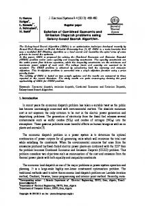
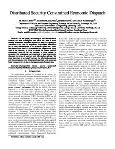
1.3 Literature Review The objective of this chapter is to review the Sequential and Parallel economic dispatch problems and the existing methods and algorithms for solution of these dispatch problems. The review divides the economic dispatch problem into Sequential and Parallel, and is done for a time period of 55 years from 1958 to 2013. The total number of 182 publications is considered. The number of publications year wise and algorithm wise is shown in the Figure 1.1 and Figure 1.2 respectively.
Fig. 1.1 Plot of Number of Publications Year Wise
2
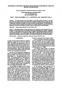
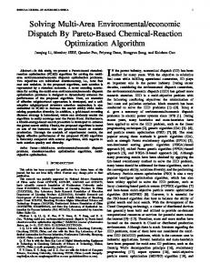
Fig. 1.2 Plot of Number of Publications Algorithm Wise (Happ, 1977) Represented a comprehensive survey of papers on optimal dispatch problem covering the period of 1920-1977 [1]. In that, the existing literature of the economic dispatch into the following main groups: classical single area, multi area economic dispatch, and optimal load flow. Classic economic dispatch of real power treats the network approximately and optimizes the generator powers when all voltages are considered constant with objective being the minimization of production costs. The classic economic dispatch was compared with the rigorous power allocation method, and it was concluded that there were no economic incentives in terms of dollars saved in order to switch to a more rigorous economic dispatch procedure. Rigorous procedures compute the incremental losses directly from the Jacobean of the Newton Raphson load flow. The work on valve point loading and environmental dispatch is also considered in his review. 3
Harmony search (Wang and Li, 2013) [2] is a new meta-heuristic optimization algorithm which imitates the music improvisation process applied by musicians. The parameters of the IHS algorithm are the Harmony Memory Size (HMS), Harmony Memory Considering Rate (HMCR), Pitch Adjusting Rate (PAR), and the Number of Improvisations (NI). Some efficient meta-heuristic search methods (Ratniyomchai et al., 2010) [3] like Genetic Algorithm, Evolutionary Programming, Adaptive Tabu Search, Particle Swarm Optimization and Improved Harmony Search are briefed and summarized. The improved harmony search method proves that it can find a place among some efficient meta-heuristic search methods in order to find a near global solution of the economic load dispatch problems. Thermal power plants play a major role in power production and they burn fossil fuels that generate toxic gases. This creates pollution for the environment. There are two objectives i) minimum cost and ii) minimum emission, converted into a single objective function determining the so called emission constrained economic dispatch (Nanda et al., 1994) [4]. It is compulsory for the electric utilities to reduce the pollution. The multi-criteria power system dispatch problem is solved using two methods in the existing literature. The bi-objective function (fuel cost and emission) is converted into single objective function by the following penalty factors: Weighted sum method (WSM) and price penalty factor method. According to (Rani et al., 2006) [5], (Jeyakumar et al., 2006) [6] the bi-criteria dispatch problem is solved using WSM method. In the papers (Dhillon et al., 1994) [7], (Tsai and Yen, 2010) [8], (Hemamalini and Simon, 2009) [9], (Thakur et al., 2006) [10], and (Ming et al., 2010) [11] the multi-criteria dispatch problem is solved using Max-Max price penalty factor method. The price penalty factor hi is the ratio between maximum fuel cost and maximum emission of corresponding generator The Combined Economic Emission Dispatch (CEED) problem is solved using Max-Max penalty factor by PSO algorithm in (Thakur et al., 2006) [10]. Solutions of the multi-objective problems are grouped into two methods namely non-interactive and interactive methods (Dhillon et al., 1994) [7]. In the non-interactive type methods a global preference function of the objectives is identified and optimized with respect to the constraints. In the interactive methods, a local preference function or trade-off among 4
objectives is identified by interacting with the decision maker, and the solution process proceeds gradually toward the globally satisfactory solution. It incorporates a sensitivity measure into multi-objective optimization, which generates a non-inferior optimal solution with respect to the objective function and the sensitivity index. The index provides useful information about the distribution of the optimal solution in the presence of variations in the model parameters defining the problem. The decision maker is able to analyze the sensitivity information conveniently. The sensitivity index is a scalar-valued quantity, regardless of the number of objectives. The most important characteristic of the sensitivity index is that a sensitivity trade-off is calculated at each non inferior point. This allows the decision maker to know the trade-offs between objective levels and parameter sensitivity. Particle Swarm Optimization (PSO) algorithm based technique for solving the emission and economic dispatch problem by using Max-Max Price penalty factor is considered. It mainly focuses on nitrogen oxides and sulfur dioxide emissions of thermal power plants. In (Tsai and Yen, 2010) [8] an Improved Particle Swarm Optimization (IPSO) is presented to solve the economic dispatch problems considering fuel cost, environmental issue, and valve point effect loading. The IPSO is developed in such a way that PSO with Constriction Factor (PSO-CF) is applied as a basic level search, which can give a good direction to the optimal global region. The IPSO introduces two operators, "Random Particles" and "Fine-Tuning" into the PSO-CF algorithm for increasing the search ability. The process of "Random Particles" will add a proper random particle into the group of particles when the solution is searched in each generation. The Max-Max penalty factor is commonly used in a Sequential and Parallel dispatch problem to combine both cost and emission functions. The Min-Max penalty factor (Krishnamurthy and Tzoneva, 2011) [12], yields better solution for the multicriteria dispatch problem in comparison to other penalty factors. The average and common penalty factor (Balamurugan and Subramanian, 2008) [13] are also used in Sequential and Parallel problem. The penalty factor approach for conversion of the multi-criteria dispatch problem in a single criterion one yields a better objective function value and calculation time for combined economic emission dispatch problem in comparison with
5
the weighted sum approach. Therefore the global solution of the Sequential and Parallel economic dispatch problem depends on the penalty factors used. The review finds that various objective functions, and constraints are used in both single area and multi-area dispatch problems as follows:
Most used objective functions are Second order fuel cost function with or without valve point loading effect.
Most used constraints are Real power balance constraint, transmission loss constraint, real power operation limits, real and reactive power flows, voltage limits, area power balance constraint, and tie-line power transfer limits constraint. It is necessary to consider the transmission loss of the power system in order to achieve accurate real power balance constraint.
Most of reference paper used Max-Max price penalty factor method.
1.4 Hypothesis The hypothesis is based on the review investigation of methods and algorithms used in the referenced papers to solve the single and multi-area economic dispatch problem.
The optimization algorithms used in economic dispatch problem solution are either based on the classical or meta-heuristic approaches so far. The hypothesis is that the classical algorithms produce better values of the criterion functions. This hypothesis is proved by development of optimization algorithms for solution of the economic dispatch problem namely, Lagrange's a classical approach and another meta-heuristic approach. The solution and computational time of the methods to solve the economic dispatch problem are compared.
The fuel cost curves with quadratic cost function and without valve point loading effect are considered. The hypothesis is that the impact of the different criterion functions on the solution of the economic dispatch problem can be analyzed and evaluated by implementation of the developed Lagrange's and meta-heuristic algorithms.
Most of the reference papers use Max-Max price penalty factor for MOEED problem solution. Thesis hypothesis is that a new price penalty factor called 'Min6
Max' in addition to that 'Max-Max' one can be developed. This newly developed price penalty factor provides less value of the fuel cost and less emission value in comparison with Max-Max one.
1.5 Economic power dispatch problem formulation The objective of solving the economic dispatch problem in electric power system is to determine the generation levels for all on-line units which minimize the total fuel cost and minimize the emission level of the system, while satisfying a set of constraints. The objective of economic dispatch is to simultaneously minimize the generation cost and to meet the load demand of a power system over some appropriate period of time while satisfying various operating constraints. The objective function of an economic dispatch problem can be formulated as, (Happ, 1977) [1]. Minimize n
n
i 1
i 1
FC Fi Pi ai Pi bi Pi Ci 2
(1.1)
Where FC
Total Fuel Cost
Fi (Pi)
Fuel cost of the unit i generator
Pi
Real power generation of a generator unit i
ai, bi, ci
Cost coefficients of generating for unit i in [$/MW2h], [$/MWh] And [$/h] respectively
n
Number of generating units
Under the constraints 1. Power balance constraints n
PG Pi PD PL i 1
(1.2)
7
Where PG
Total power generation of the system
PD
Total demand of the system
PL
Total transmission loss of the system
2. The transmission loss can be expressed as, (Dhillon et al, 1994) [7] n
n
n
PL PiBijPj BoiPi Boo i 1 j 1
(1.3)
i 1
Where Pi
Active power generation of unit i
Pj
Active power generation of unit j
Bij, Boi, Boo
Transmission loss coefficients
3. Generator operational constraints
Pi min Pi Pi max
(1.4)
Where Pimin
Minimum value of real power allowed at a generator i
Pimax
Maximum value of real power allowed at a generator i
The various pollutants like sulphur dioxide, nitrogen oxide and carbon dioxide are released as a result of operation of the thermal power plants. Reduction of these Pollutants is compulsory for every generating unit. To achieve this goal new criteria are included in formulation of the economic dispatch problem as Follows (Tsai and Yen, 2010) [8]. n
ET d i Pi ei Pi f i i 1
2
(1.5)
Where ET
Total Emission Value
8
Emission coefficients of generating unit i [kg/MW2h], [kg/MWh]
di, ei, fi
And [kg/h] respectively A multi-objective optimization is converted into a single objective optimization one called Combined Economic Emission Dispatch (CEED) problem by introducing price penalty factor hi to the various pollutants (Balamurugan and Subramanian, 2008) [13]. n
FT ai Pi bi Pi ci hi di Pi ei Pi f i i 1
2
2
(1.6)
Where FT
Total CEED Cost
The role of price penalty factor is to transfer the physical meaning of emission criterion from weight of the emission to the fuel cost for the emission. The difference between these penalty factors is in the weight of the fuel cost for emission in the final optimal fuel cost for generation and emission. The price penalty factor for multi-objective dispatch problem (Balamurugan and Subramanian, 2008) [13] is formulated taking the ratio fuel cost to emission value of the corresponding generators as follows: Min-Max price penalty factor is described as:
a P h d P
2 i i min 2 i i max
i
bi Pi min ci 2 ei Pi max f i
[$/hr]
(1.7)
Max-Max price penalty factor is described as:
a P h d P
2 i i max 2 i i max
i
bi Pi max ci 2 ei Pi max f i
[$/hr]
(1.8)
1.6 Assumptions The research is conducted on the basis of the assumptions used to solve the Multi-objective economic emission dispatch using Sequential and Parallel method, they are:
For simplicity the power demand of the power system is considered as constant for some period of time for which the economic dispatch problem is solved. But in reality the power demand is changing in real-time in respect to the load consumed by the consumers. 9
It is a common practice for including the effect of transmission losses in the economic dispatch problem to express the total transmission loss as a quadratic function of the generator power outputs given by Kron's formulae (Dhillon et al, 1994) [7] but in reality the active power transmission losses are calculated using the power flow equations of the power system.
The tie-lines are not considered in the emission function of the interconnected power system because the transmission of power does not create chemical pollution.
Lagrange's method follows the gradient procedure to obtain the global solution.
Lagrange's method needs the initial guess of the Lagrange‘s multiplier λ to start the search process.
Meta-heuristic method needs the initial guess of constant and random numbers to start the search process.
Meta-heuristic method does not require that the optimization problem be differentiable as like classic optimization methods such as Lagrange's, gradient descent and quasi-newton methods.
Metaheuristic algorithm do not guarantee an optimal solution is ever found since it does not use the gradient procedure of the problem being optimized.
1.7 Thesis Organization This thesis titled as “A Multi-objective Economic Emission Dispatch Problem Soluation using a Sequential and Parallel Method” is divided into six chapters, the brief discussion is as follows: Chapter-I, a brief introduction on Multi-objective Economic Emission Dispatch Problem is given. Awareness of the problem, Hypothesis, problem formulation, Assumption is also given. The brief literature review is done for Multi-objective Economic Emission Dispatch Problem. Organization of the thesis is also discussed. Chapter-II, Particle swarm optimization (PSO) technique and its algorithm has been discussed. A Multi-objective Economic Emission Dispatch Problem Solution using a
10
Sequential and Parallel Method problem has been solved for the IEEE 30 bus with 6 generator system by PSO technique with Price Penalty Factor Approach. Chapter-III, BAT algorithm (BA) technique and its algorithm has been discussed. A Multiobjective Economic Emission Dispatch Problem Solution using a Sequential and Parallel Method problem has been solved for the IEEE 30 bus with 6 generator system by BA technique with Price Penalty Factor Approach. Chapter-IV, Firefly algorithm (FA) technique and its algorithm has been discussed. A Multi-objective Economic Emission Dispatch Problem Solution using a Sequential and Parallel Method problem has been solved for the IEEE 30 bus with 6 generator system by FA technique with Price Penalty Factor Approach. Chapter-V, Flower Pollination algorithm (FPA) technique and its algorithm has been discussed. A Multi-objective Economic Emission Dispatch Problem Solution using a Sequential and Parallel Method problem has been solved for the IEEE 30 bus with 6 generator system by FPA technique with Price Penalty Factor Approach. Chapter-VI, Ant Lion Optimizer (ALO) technique and its algorithm has been discussed. A Multi-objective Economic Emission Dispatch Problem Solution using a Sequential and Parallel Method problem has been solved for the IEEE 30 bus with 6 generator system by ALO technique with Price Penalty Factor Approach. Chapter-VII, Grey Wolf Optimizer (GWO) technique and its algorithm has been discussed. A Multi-objective Economic Emission Dispatch Problem Solution using a Sequential and Parallel Method problem has been solved for the IEEE 30 bus with 6 generator system by GWO technique with Price Penalty Factor Approach. Chapter-VIII, Multi-Verse Optimizer (MVO) technique and its algorithm has been discussed. A Multi-objective Economic Emission Dispatch Problem Solution using a Sequential and Parallel Method problem has been solved for the IEEE 30 bus with 6 generator system by MVO technique with Price Penalty Factor Approach.
11
Chapter-IX, Dragonfly algorithm (DA) technique and its algorithm has been discussed. A Multi-objective Economic Emission Dispatch Problem Solution using a Sequential and Parallel Method problem has been solved for the IEEE 30 bus with 6 generator system by DA technique with Price Penalty Factor Approach. Chapter-X, Lagrange’s algorithm (LA) technique and its algorithm has been discussed. A Multi-objective Economic Emission Dispatch Problem Solution using a Sequential and Parallel Method problem has been solved for the IEEE 30 bus with 6 generator system by LA technique with Price Penalty Factor Approach. Chapter-XI, deals with the conclusion and the future scope of the work.
12
CHAPTER-2 PARTICLE SWARM OPTIMIZATION 2.1 Introduction A Multi-objective Economic Emission Dispatch problem solution using a Sequential and Parallel method by Particle swarm optimization algorithm shown in this Chapter. The particle swarm optimization algorithm (PSO) was first described by James Kennedy and Russell C. Eberhart in 1995 [14]. This algorithm is inspired by simulation of social psychological expression of birds and fishes.
2.2 Particle Swarm Optimization The particle with the best fitness value is considered the leader of the swarm, and guides the other members to promising areas of the search space. Each particle is influenced on its search direction by cognitive (i.e. its own best position found so far, called Pbest) and social (i.e. the position of the leader of the swarm named Gbest) information. At each iteration (generation) of the process, the leader of the swarm is updated. These two elements: Pbest and Gbest, besides the current position of particle X, are used to calculate its new velocity v(t+1) based on its current velocity v(t) (search direction) as follow equations (2.1) and (2.2). vijt 1 wvijt c1R1 ( Pbest t X t ) c2 R2 (Gbest t X t )
(2.1)
X t 1 X t vt 1 (i=1, 2...NP) and (j=1, 2...NG)
(2.2)
Where
w wmax
( wmax wmin )* iteration max iteration
, No. of iteration=2000.
(2.3)
wmax =0.4 and wmin =0.9, NP=No. of Particles=10 and NG=No. of Generators=6. vijt , vijt 1 Is the velocity of jth member of ith particle at iteration number (t) and (t+1).
(Usually C1=C2=2), R1 and R2 Random number (0, 1). 13
2.3 Flow chart of Particle Swarm Optimization
Fig. 2.1 Flow Chart for PSO Algorithm
14
2.4 Simulation Results The Multi-Objective Economic Emission Dispatch (MOEED) problem is formulated in Chapter 1. The fuel cost equation is given in (1.1) and is solved subject to the constraints (1.2), (1.3.), and (1.4). The emission function is given in (1.5) and the price penalty factors (1.7) and (1.8) are used to formulate Multi Objective into the single objective function (1.6) of the MOEED problem. PSO algorithm described in section 2.2 and section 2.3 is applied for the solution of the MOEED problem using Sequential and parallel input for IEEE 30 bus with 6 generator system and the data of fuel cost, emission coefficients, loss coefficient and generator limits are given in Appendix A (Gnanadass, 2005) [15]. The various power demands (PD) of 125 to 250 [MW] are considered. The calculations are carried out in the Matlab software environment. The optimal solution of the MOEED problem in Sequential and parallel input using PSO algorithm is given in Tables 2.1, Tables 2.2 Fig. 2.2, Fig. 2.3, Fig. 2.4 and Fig. 2.5 using “Min-Max” and “Max-Max” Penalty factors respectively. PD
P1
P2
P3
P4
P5
P6
PL
FC
ET
FT
[MW] [MW] [MW] [MW] [MW] [MW] [MW] [MW] [$/hr] [Kg/hr] [$/hr] 125
20.10
39.09
18.74
14.92
20.12
12.75 0.758 340.82 184.64 424.80
150
58.11
26.01
25.82
11.97
10.56
19.03 1.530 394.53 167.32 472.74
175
81.21
31.34
18.90
16.84
10.12
19.06 2.492 456.75 184.22 541.57
200
98.77
44.49
15.46
10.04
16.29
18.67 3.750 530.82 219.32 627.29
225
115.29 42.86
20.66
18.94
15.05
16.83 4.659 607.94 252.19 716.92
250
141.06 52.57
19.68
16.55
12.65
14.19 6.736 686.73 317.20 816.30
Table 2.1 MOEED problem solution using PSO algorithm Min-Max Penalty factor result 15
PD
P1
P2
P3
P4
P5
P6
PL
FC
ET
FT
[MW] [MW] [MW] [MW] [MW] [MW] [MW] [MW] [$/hr] [Kg/hr] [$/hr] 125
34.54
28.32
17.59
19.56
10.88
14.93 0.848 326.88
162.54 674.76
150
53.37
27.86
16.85
16.26
22.09
14.93 1.377 398.29
168.45 760.43
175
79.42
25.62
20.76
16.57
14.63
20.29 2.305 463.109 182.52 851.69
200
98.04
34.51
21.34
16.86
14.05
18.58 3.408 531.87
212.13 972.50
225
107.54
44.06
18.90
26.81
19.04
12.89 4.268 612.98
250.29 1123.2
250
124.63
47.71
24.08
25.06
16.51
17.52 5.539 694.51
291.97 1282.5
Table 2.2 MOEED problem solution using PSO algorithm Max-Max Penalty factor result
Fig. 2.2 Plot of Fuel Cost Vs. Power Demand using PSO algorithm
16
Fig. 2.3 Plot of Emission value Vs. Power Demand using PSO algorithm
Fig. 2.4 Plot of Power Loss Vs. Power Demand using PSO algorithm
17
Fig. 2.5 Plot of CEED Fuel Cost Vs. Power Demand using PSO algorithm
2.5 Discussion and Conclusion The obtained results from Table 2.1, Table 2.2, Fig. 2.2, Fig. 2.3, Fig. 2.4 and Fig. 2.5 display that the “Min-Max” price penalty factor have good result for MOEED using a Sequential and parallel method with PSO and compare to the “Max-Max “price penalty factors. It can be represented that: The optimal overall cost Combined Economic Emission Dispatch (CEED) and fuel cost are less when using “Min-Max” Price penalty factor in Place of “Max-Max” price penalty factors. The “Max-Max” price penalty factor is good to yield a minimum emission and power loss values with respect of “Min-Max” price penalty factors. In Sequential and Parallel method obtained result will be same because in Sequential approach Power demand (input) given one by one and obtained result but in Parallel method approach Power demand (input) given at a one time and all result obtained one time run process. 18
CHAPTER-3 BAT ALGORITHM 3.1 Introduction A Multi-objective Economic Emission Dispatch problem solution using a Sequential and parallel method by BAT algorithm shown in this Chapter. BAT algorithm (BA) [16] is a Swarm Intelligence based optimization technique developed by (Xin-She Yang, 2010), inspired by the echolocation behavior of micro bats. BAT algorithm (BA) first time used frequency tuning.
3.2 BAT Algorithm BA simulations, we use virtual bats naturally. We have used to BAT motion rules how their positions Xi and velocities Vi in a d-dimensional search space are updated. The new solutions Xit and velocities Vit at time step t are given by equation (3.1) and equation (3.2):
fi f min f max f min *
(3.1)
vi t vi t 1 x i t – x* *fi
(3.2)
Where β ϵ [0, 1] is a random vector drawn from a uniform distribution. Here X* is the current global best location (solution) which is located after comparing all the solutions among all the n bats. As the product λifi is the velocity increment, we can use either fi (or λi) to adjust the velocity change while fixing the other factor λi (fi), depending on the type of the problem of interest. For the local search part, once a solution is selected among the current best solutions, a new solution for each bat is generated locally using random walk given by equation (3.3).
xnew xold At
(3.3)
Where ε ϵ [−1, 1] is a random number, while At = 0 from a Levy distribution in equation (5.2):
πλ ) 2 1 , (S>>S0>>0) π S1 λ
λΓ(λ)sin( L~
(5.2)
31
Here, Γ (λ) = Standard gamma function, and this distribution is valid for large steps s > 0. Then, model the local pollination, both Rule 2 and Rule 3 can represented equation (5.3):
x it 1 x it U (x tj x kt )
(5.3)
Where x tj and x kt are pollen from different flowers of the same plant species.
5.3 Pseudo-codes of Flower Pollination Algorithm
Fig. 5.1 Pseudo-codes for FPA Algorithm 32
5.4 Simulation Results The Multi-Objective Economic Emission Dispatch (MOEED) problem is formulated in Chapter 1. The fuel cost equation is given in (1.1) and is solved subject to the constraints (1.2), (1.3.), and (1.4). The emission function is given in (1.5) and the price penalty factors (1.7) and (1.8) are used to formulate Multi Objective into the single objective function (1.6) of the MOEED problem. FPA algorithm described in section 5.2 and section 5.3 is applied for the solution of the MOEED problem using Sequential and parallel input for IEEE 30 bus with 6 generator system and the data of fuel cost, emission coefficients, loss coefficient and generator limits are given in Appendix A (Gnanadass, 2005) [15]. The various power demands (PD) of 125 to 250 [MW] are considered. The calculations are carried out in the Matlab software environment. The optimal solution of the MOEED problem in Sequential and parallel input using FPA algorithm is given in Tables 5.1, Tables 5.2 Fig. 5.2, Fig. 5.3, Fig. 5.4 and Fig. 5.5 using “Min-Max” and “Max-Max” Penalty factors respectively. PD
P1
P2
P3
P4
P5
P6
PL
FC
ET
FT
[MW] [MW] [MW] [MW] [MW] [MW] [MW] [MW] [$/hr] [Kg/hr] [$/hr] 125
59.24
20.00
15.00
10.00
10.00
12.00
1.24
308.15 144.52 377.18
150
78.86
26.22
15.00
10.00
10.00
12.00
2.09
373.49 162.22 448.51
175
94.71
30.01
19.11
11.14
10.40
12.46
2.95
445.77 187.94 538.46
200
113.45 39.55
19.16
10.09
10.00
12.00
4.28
519.68 227.68 616.96
225
127.28 44.26
20.65
15.00
11.11
12.03
5.35
601.20 267.50 713.06
250
138.82 48.69
22.32
19.04
13.70
13.83
6.42
687.09 310.06 815.18
Table 5.1 MOEED problem solution using FPA algorithm Min-Max Penalty factor result 33
PD
P1
P2
P3
P4
P5
P6
PL
FC
ET
FT
[MW] [MW] [MW] [MW] [MW] [MW] [MW] [MW] [$/hr] [Kg/hr] [$/hr] 125
55.34
21.55
15.95
10.58
10.15
12.64
1.24
309.93
144.51 624.07
150
79.37
25.46
15.08
10.00
10.02
12.12
2.08
373.68
162.14 716.33
175
90.15
31.49
17.24
14.09
12.38
12.40
2.78
448.59
185.69 835.82
200
100.85
36.57
19.22
17.37
14.95
14.55
3.55
528.03
214.33 969.90
225
110.20
41.07
20.90
21.63
17.95
17.56
4.34
612.12
247.25 1117.7
250
119.21
46.10
23.66
25.10
20.78
20.34
5.20
699.61
285.29 1279.1
Table 5.2 MOEED problem solution using FPA algorithm Max-Max Penalty factor result
Fig. 5.2 Plot of Fuel Cost Vs. Power Demand using FPA algorithm 34
Fig. 5.3 Plot of Emission value Vs. Power Demand using FPA algorithm
Fig. 5.4 Plot of Power Loss Vs. Power Demand using FPA algorithm
35
Fig. 5.5 Plot of CEED Fuel Cost Vs. Power Demand using FPA algorithm
5.5 Discussion and Conclusion The obtained results from Tables 5.1, Tables 5.2 Fig. 5.2, Fig. 5.3, Fig. 5.4 and Fig. 5.5 display that the “Min-Max” price penalty factor have good result for MOEED using a Sequential and parallel method with FPA and compare to the “Max-Max “price penalty factors. It can be represented that: The optimal overall cost Combined Economic Emission Dispatch (CEED) and fuel cost are less when using “Min-Max” Price penalty factor in Place of “Max-Max” price penalty factors. The “Max-Max” price penalty factor is good to yield a minimum emission and power loss values with respect of “Min-Max” price penalty factors. In Sequential and Parallel method obtained result will be same because in Sequential approach Power demand (input) given one by one and obtained result but in Parallel method approach Power demand (input) given at a one time and all result obtained one time run process.
36
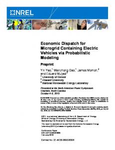
CHAPTER-6 ANT LION OPTIMIZER 6.1 Introduction A Multi-objective Economic Emission Dispatch problem solution using a Sequential and parallel method by Ant Lion Optimizer shown in this Chapter. The Ant Lion Optimizer (ALO) is a Swarm Intelligence based optimization technique that was first described by Seyedali Mirjalili in 2015 [19]. This algorithm is inspired by hunting mechanism of ant lions in nature.
6.2 Ant Lion Optimizer The Ant Lion Optimizer (ALO) algorithm mimics the build trap and hunting mechanism of ant lions in nature. In ant lion have Five main steps of hunting prey such as the (1) random walk of ants, (2) building traps, (3) entrapment of ants in traps, (4) catching preys, and (5) re-building traps are implemented to perform optimization information shown in figure (6.1).
Fig. 6.1 Hunting Mechanism of Ant Lions
37
Each of the behaviors is mathematically modeled as: The Random walks of ants is calculated as follows equation (6.1)
( xit ai ) *(di cit ) x ci (dit ai ) t i
(6.1)
Where, ai is the minimum of random walk of ith variable, bi is the Maximum of random walk in ith variable. The Trapping in ant lion’s pits is calculated as follows equation (6.2) and equation (6.3) (6.2) (6.3) The Sliding ants towards ant lion calculated as follows equation (6.4) and equation (6.5) ct ct (6.4) I dt
dt I
(6.5)
Where, I is a ratio, ct is the minimum of all variables at tth iteration, and dt indicates the vector including the maximum of all variables at tth iteration. Catching prey and re-building the pits calculated as follows equation (6.6)
Antliontj Antit if f
Ant t i
f ( Antliontj )
(6.6)
Where, t shows the current iteration, 𝐴𝑛𝑡𝑙𝑖𝑜𝑛𝑡𝑖 shows the position of selected jth ant lion at tth iteration, and 𝐴𝑛𝑡𝑡𝑖 indicates the position of ith ant at tth iteration. Elitism of ant lion calculated using roulette wheel as follows equation (6.7)
RAt REt Ant 2 t i
(6.7)
38
6.3 Pseudo-codes of Ant Lion Optimizer
Fig. 6.2 Pseudo-code of Ant Lion Optimizer 39
6.4 Simulation Results The Multi-Objective Economic Emission Dispatch (MOEED) problem is formulated in Chapter 1. The fuel cost equation is given in (1.1) and is solved subject to the constraints (1.2), (1.3.), and (1.4). The emission function is given in (1.5) and the price penalty factors (1.7) and (1.8) are used to formulate Multi Objective into the single objective function (1.6) of the MOEED problem. ALO algorithm described in section 6.2 and section 6.3 is applied for the solution of the MOEED problem using Sequential and parallel input for IEEE 30 bus with 6 generator system and the data of fuel cost, emission coefficients, loss coefficient and generator limits are given in Appendix A (Gnanadass, 2005) [15]. The various power demands (PD) of 125 to 250 [MW] are considered. The calculations are carried out in the Matlab software environment. The optimal solution of the MOEED problem in Sequential and parallel input using ALO algorithm is given in Tables 6.1, Tables 6.2 Fig. 6.3, Fig. 6.4, Fig. 6.5 and Fig. 6.6 using “Min-Max” and “Max-Max” Penalty factors respectively. PD
P1
P2
P3
P4
P5
P6
PL
FC
ET
FT
[MW] [MW] [MW] [MW] [MW] [MW] [MW] [MW] [$/hr] [Kg/hr] [$/hr] 125
59.24
20.00
15.00
10.00
10.00
12.00
1.24
308.15 144.52 377.18
150
79.26
25.83
15.00
10.00
10.00
12.00
2.10
373.58 162.21 448.51
175
96.61
32.86
16.63
10.00
10.00
12.00 3.106 443.98 190.34 528.55
200
114.09 39.32
18.88
10.00
10.00
12.00
4.30
519.49 228.15 616.94
225
127.64 44.43
20.77
14.15
11.37
12.00
5.38
601.09 268.10 713.05
250
138.80 48.70
22.33
19.10
13.64
13.83
6.42
687.09 310.06 815.17
Table 6.1 MOEED problem solution using ALO algorithm Min-Max Penalty factor result 40
PD
P1
P2
P3
P4
P5
P6
PL
FC
ET
FT
[MW] [MW] [MW] [MW] [MW] [MW] [MW] [MW] [$/hr] [Kg/hr] [$/hr] 125
59.24
20.00
15.00
10.00
10.00
12.00
1.24
308.15
144.52 619.25
150
79.52
25.57
15.00
10.00
10.00
12.00
2.10
373.47
162.20 716.15
175
91.59
31.77
17.07
13.45
11.93
12.00
2.84
447.45
186.53 835.64
200
100.93
36.59
19.24
17.38
14.88
14.51
3.55
527.95
214.39 969.89
225
110.09
41.32
21.40
21.25
17.81
17.43
4.34
612.04
247.25 1117.6
250
119.24
46.07
23.58
25.17
20.74
20.37
5.21
699.57
285.31 1279.1
Table 6.2 MOEED problem solution using ALO algorithm Max-Max Penalty factor result
Fig. 6.3 Plot of Fuel Cost Vs. Power Demand using ALO algorithm 41
Fig. 6.4 Plot of Emission value Vs. Power Demand using ALO algorithm
Fig. 6.5 Plot of Power Loss Vs. Power Demand using ALO algorithm
42
Fig. 6.6 Plot of CEED Fuel Cost Vs. Power Demand using ALO algorithm
6.5 Discussion and Conclusion The obtained results from Tables 6.1, Tables 6.2 Fig. 6.3, Fig. 6.4, Fig. 6.5 and Fig. 6.6 display that the “Min-Max” price penalty factor have good result for MOEED using a Sequential and parallel method with ALO and compare to the “Max-Max “price penalty factors. It can be represented that: The optimal overall cost Combined Economic Emission Dispatch (CEED) and fuel cost are less when using “Min-Max” Price penalty factor in Place of “Max-Max” price penalty factors. The “Max-Max” price penalty factor is good to yield a minimum emission and power loss values with respect of “Min-Max” price penalty factors. In Sequential and Parallel method obtained result will be same because in Sequential approach Power demand (input) given one by one and obtained result but in Parallel method approach Power demand (input) given at a one time and all result obtained one time run process.
43
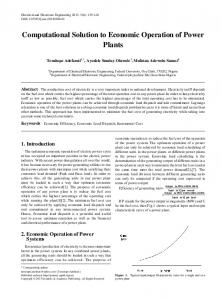
CHAPTER-7 GREY WOLF OPTIMIZER 7.1 Introduction A Multi-objective Economic Emission Dispatch problem solution using a Sequential and parallel method by Grey Wolf Optimizer shown in this Chapter. The Grey Wolf Optimizer (GWO) is a met heuristics based optimization technique that was first described by Seyedali Mirjalili, Seyed Mohammad Mirjalili and Andrew Lewis in 2013 [20]. This algorithm is inspired by hunting behavior of grey wolves.
7.2 Grey Wolf Optimizer The Grey Wolf Optimizer (GWO) algorithm mimics the leadership hierarchy and hunting mechanism of grey wolves in nature. Four types of grey wolves such as alpha (first fittest solution), beta (second fittest solution), delta (third fittest solution), and omega (fourth fittest solution) are employed for simulating the leadership hierarchy. In addition, main steps of hunting, searching for prey, encircling prey, and attacking prey, are implemented to perform optimization information shown in figure (7.1).
Fig. 7.1 Hunting Mechanism of Grey Wolves 44
Each of the behaviors is mathematically modeled as: The Encircling prey is calculated as follows equation (7.1) and equation (7.2)
D | C* X p t X (t ) |
(7.1)
X t 1 X p t A* D
(7.2)
Where, t=current iteration, X p = position vector of the prey, X = position vector of grey
wolf, A, C coefficient vectors are calculated as follows equation (7.3) and equation (7.4)
A 2 a* r1 a
(7.3)
C 2 r2
(7.4)
Where, components of a are linearly decreased from 2 to 0 over the course of iterations and r1, r2 are random vectors in [0, 1]. The Hunting process is calculated as follows equation (7.3) to equation (7.11)
D | C1* X X |
(7.5)
D | C2 * X X |
(7.6)
D | C3 * X X |
(7.7)
X 1 X A1*( D )
(7.8)
X 2 X A2 *( D )
(7.9)
X 3 X A3 *( D )
(7.10)
X X2 X3 X t 1 1 3
(7.11)
45
7.3 Pseudo-codes of Grey Wolf Optimizer
Fig. 7.2 Pseudo-code of Grey Wolf Optimizer 46
7.4 Simulation Results The Multi-Objective Economic Emission Dispatch (MOEED) problem is formulated in Chapter 1. The fuel cost equation is given in (1.1) and is solved subject to the constraints (1.2), (1.3.), and (1.4). The emission function is given in (1.5) and the price penalty factors (1.7) and (1.8) are used to formulate Multi Objective into the single objective function (1.6) of the MOEED problem. GWO algorithm described in section 7.2 and section 7.3 is applied for the solution of the MOEED problem using Sequential and parallel input for IEEE 30 bus with 6 generator system and the data of fuel cost, emission coefficients, loss coefficient and generator limits are given in Appendix A (Gnanadass, 2005) [15]. The various power demands (PD) of 125 to 250 [MW] are considered. The calculations are carried out in the Matlab software environment. The optimal solution of the MOEED problem in Sequential and parallel input using GWO algorithm is given in Tables 7.1, Tables 7.2 Fig. 7.3, Fig. 7.4, Fig. 7.5 and Fig. 7.6 using “Min-Max” and “Max-Max” Penalty factors respectively. PD
P1
P2
P3
P4
P5
P6
PL
FC
ET
FT
[MW] [MW] [MW] [MW] [MW] [MW] [MW] [MW] [$/hr] [Kg/hr] [$/hr] 125
58.76
20.51
15.00
10.00
10.00
12.00
1.24
308.26 144.71 377.33
150
79.54
25.54
15.01
10.00
10.00
12.00
2.10
373.50 162.21 448.55
175
96.14
34.54
15.45
10.03
10.00
12.00
3.13
444.29 190.95 528.98
200
115.55 37.87
18.77
10.04
10.08
12.00
4.33
519.23 228.63 617.01
225
127.76 43.45
19.88
14.52
12.31
12.42
5.35
601.29 267.04 713.71
250
137.70 48.94
22.24
18.37
14.29
14.74
6.36
687.43 308.20 814.97
Table 7.1 MOEED problem solution using GWO algorithm Min-Max Penalty factor result 47
PD
P1
P2
P3
P4
P5
P6
PL
FC
ET
FT
[MW] [MW] [MW] [MW] [MW] [MW] [MW] [MW] [$/hr] [Kg/hr] [$/hr] 125
59.24
20.00
15.00
10.00
10.00
12.00
1.24
308.19
144.53 619.31
150
78.83
26.22
15.00
10.06
10.00
12.00
2.09
373.71
162.25 716.47
175
91.92
31.66
17.06
13.35
11.80
12.02
2.85
447.22
186.64 835.52
200
100.72
36.47
19.71
16.73
14.98
14.98
3.54
528.32
214.37 970.16
225
110.14
41.64
21.40
21.36
17.29
17.46
4.35
611.69
247.48 1117.5
250
118.52
45.18
23.69
26.01
20.77
21.00
5.15
700.65
284.52 1279.5
Table 7.2 MOEED problem solution using GWO algorithm Max-Max Penalty factor result
Fig. 7.3 Plot of Fuel Cost Vs. Power Demand using GWO algorithm 48
Fig. 7.4 Plot of Emission value Vs. Power Demand using GWO algorithm
Fig. 7.5 Plot of Power Loss Vs. Power Demand using GWO algorithm
49
Fig. 7.6 Plot of CEED Fuel Cost Vs. power demand using GWO algorithm
7.5 Discussion and Conclusion The obtained results from Tables 7.1, Tables 7.2 Fig. 7.3, Fig. 7.4, Fig. 7.5 and Fig. 7.6 display that the “Min-Max” price penalty factor have good result for MOEED using a Sequential and parallel method with GWO and compare to the “Max-Max “price penalty factors. It can be represented that: The optimal overall cost Combined Economic Emission Dispatch (CEED) and fuel cost are less when using “Min-Max” Price penalty factor in Place of “Max-Max” price penalty factors. The “Max-Max” price penalty factor is good to yield a minimum emission and power loss values with respect of “Min-Max” price penalty factors. In Sequential and Parallel method obtained result will be same because in Sequential approach Power demand (input) given one by one and obtained result but in Parallel method approach Power demand (input) given at a one time and all result obtained one time run process.
50
CHAPTER-8 MULTI-VERSE OPTIMIZER 8.1 Introduction A Multi-objective Economic Emission Dispatch problem solution using a Sequential and parallel method by Multi-Verse Optimizer shown in this Chapter. The Multi-Verse Optimizer (MVO) is a Physics theory based optimization technique that was first described by Seyedali Mirjalili in 2015 [21]. This algorithm is inspired by Multi-Verse and Cosmology theory in Universe.
8.2 Multi-verse Optimizer The Multi-Verse Optimizer (MVO) algorithm are based on three concepts in cosmology: white hole, black hole, and wormhole. The mathematical models of these three concepts are developed to perform exploration, exploitation, and local search respectively information shown in figure (6.1).
Fig. 8.1 Conceptual Model of Multi-Verse Optimizer 51
During optimization, the following rules are applied to the universes of MVO: 1. The higher inflation rate, the higher probability of having white hole. 2. The higher inflation rate, the lower probability of having black holes. 3. Universes with higher inflation rate tend to send objects through white holes. 4. Universes with lower inflation rate tend to receive more objects through black holes. 5. The objects in all universes may face random movement towards the best universe via wormholes regard- less of the inflation rate. 6. Wormhole existence probability (WEP) and traveling distance rate variation (TDR) shown in figure (8.2) Each of the concept is mathematically modeled explained in Pseudo-codes section (8.3)
Fig. 8.2 Wormhole existence probability Vs. traveling distance rate variation
52
8.3 Pseudo-codes of Multi-Verse Optimizer
Fig. 8.3 Pseudo-code of Multi-Verse Optimizer 53
8.4 Simulation Results The Multi-Objective Economic Emission Dispatch (MOEED) problem is formulated in Chapter 1. The fuel cost equation is given in (1.1) and is solved subject to the constraints (1.2), (1.3.), and (1.4). The emission function is given in (1.5) and the price penalty factors (1.7) and (1.8) are used to formulate Multi Objective into the single objective function (1.6) of the MOEED problem. MVO algorithm described in section 8.2 and section 8.3 is applied for the solution of the MOEED problem using Sequential and parallel input for IEEE 30 bus with 6 generator system and the data of fuel cost, emission coefficients, loss coefficient and generator limits are given in Appendix A (Gnanadass, 2005) [15]. The various power demands (PD) of 125 to 250 [MW] are considered. The calculations are carried out in the Matlab software environment. The optimal solution of the MOEED problem in Sequential and parallel input using MVO algorithm is given in Tables 8.1, Tables 8.2, Fig. 8.4, Fig. 8.5, Fig. 8.6 and Fig. 8.7 using “Min-Max” and “Max-Max” Penalty factors respectively. PD
P1
P2
P3
P4
P5
P6
PL
FC
ET
FT
[MW] [MW] [MW] [MW] [MW] [MW] [MW] [MW] [$/hr] [Kg/hr] [$/hr] 125
59.25
20.00
15.00
10.00
10.00
12.00
1.25
308.21 144.54 377.24
150
79.27
24.73
16.03
10.00
10.04
12.00
2.08
373.82 162.00 448.83
175
97.66
31.48
16.59
10.35
10.00
12.00
3.11
444.00 190.31 528.69
200
113.03 39.16
18.44
11.59
10.00
12.01
4.23
520.03 226.65 617.50
225
126.96 41.90
20.71
15.40
12.76
12.48
5.25
601.73 264.79 713.54
250
139.35 49.07
22.33
18.17
13.93
13.57
6.47
686.89 311.11 815.45
Table 8.1 MOEED problem solution using MVO algorithm Min-Max Penalty factor result 54
PD
P1
P2
P3
P4
P5
P6
PL
FC
ET
FT
[MW] [MW] [MW] [MW] [MW] [MW] [MW] [MW] [$/hr] [Kg/hr] [$/hr] 125
59.23
20.00
15.00
10.00
10.00
12.00
1.24
308.15
144.52 619.28
150
78.95
26.15
15.00
10.00
10.00
12.00
2.09
373.53
162.23 716.45
175
91.47
32.09
16.82
13.53
11.91
12.01
2.85
447.49
186.61 835.78
200
101.28
37.04
18.64
16.17
15.57
14.83
3.58
527.83
214.64 970.01
225
110.29
41.64
22.00
21.28
17.14
16.97
4.35
611.54
247.66 1117.7
250
119.35
45.79
23.68
25.39
20.73
20.24
5.20
699.55
285.31 1279.1
Table 8.2 MOEED problem solution using MVO algorithm Max-Max Penalty factor result
Fig. 8.4 Plot of Fuel Cost Vs. Power Demand using MVO algorithm 55
Fig. 8.5 Plot of Emission value Vs. Power Demand using MVO algorithm
Fig. 8.6 Plot of Power Loss Vs. Power Demand using MVO algorithm
56
Fig. 8.7 Plot of CEED Fuel Cost Vs. power demand using MVO algorithm
8.5 Discussion and Conclusion The obtained results from Tables 8.1, Tables 8.2, Fig. 8.4, Fig. 8.5, Fig. 8.6 and Fig. 8.7 display that the “Min-Max” price penalty factor have good result for MOEED using a Sequential and parallel method with MVO and compare to the “Max-Max “price penalty factors. It can be represented that: The optimal overall cost Combined Economic Emission Dispatch (CEED) and fuel cost are less when using “Min-Max” Price penalty factor in Place of “Max-Max” price penalty factors. The “Max-Max” price penalty factor is good to yield a minimum emission and power loss values with respect of “Min-Max” price penalty factors. In Sequential and Parallel method obtained result will be same because in Sequential approach Power demand (input) given one by one and obtained result but in Parallel method approach Power demand (input) given at a one time and all result obtained one time run process.
57
CHAPTER-9 DRAGONFLY ALGORITHM 9.1 Introduction A Multi-objective Economic Emission Dispatch problem solution using a Sequential and parallel method by Dragonfly algorithm shown in this Chapter. The Dragonfly algorithm (DA) is a Swarm Intelligence based optimization technique that was first described by Seyedali Mirjalili in May, 2015 [22]. This algorithm is inspired by Static and Dynamic swarming behaviors of dragonfly in nature.
9.2 Dragonfly Algorithm Dragonflies create sub swarms and fly over different areas in a static swarm, which is the main objective of the exploration phase. In the static swarm, however, dragonflies fly in bigger swarms and along one direction, which is favourable in the exploitation phase. A conceptual model of the dynamic and static swarms are illustrated in the following figure (9.1).
Fig. 9.1 Dynamic versus Static dragonfly swarms
58
We used five concepts allowed me to simulate the behavior of dragonflies in both dynamic and static swarms. The following figures (9.2) shows how my proposed model moves the individuals around the search space with respect to each other as well as food source and enemy. Please note that the green asterisk is food source, the red asterisk indicates the enemy, black circles are individuals, and blue lines are the step vector of the dragonflies.
Fig. 9.2 Dragonfly Algorithm principle Each of the behaviors is mathematically modeled as: The separation is calculated as follows equation (9.1) N
Si=- X Xj
(9.1)
j 1
59
The Alignment is calculated as follows equation (9.2) N
X
j
Ai=
j 1
(9.2)
N
The cohesion is calculated as follows equation (9.3) N
X
j
Ci=
j 1
N
X
(9.3)
Attraction towards a food source is calculated as follows equation (9.4) Fi=X+ - X
(9.4)
Distraction outwards an enemy is calculated as follows equation (9.5) Ei=X- + X
(9.5)
Where X=Position of the current individuals, N=number of neighboring individuals, X+=positions of food source, X-=positions of enemy Step vector is calculated using equation (9.6)
∆Xt+1 = (sSi+aAi+cCi+fFi+eEi)+w∆Xt
(9.6)
Position vector is calculated using equation (9.7)
Xt+1=Xt +∆Xt+1
(9.7)
And Position of dragonfly updated using equation (9.8)
Xt+1=Xt +Levy(x)*Xt
(9.8)
Where s=separation weight. a=alignment weight. c=cohesion weight. 60
f=food weight. e=enemy weight. w=inertia weight. t=iteration counter. No. of iteration=2000. No. of Dragonfly=40. d=dimension of position vectors that levy flight step calculated
9.3 Pseudo-codes of Dragonfly Algorithm
Fig. 9.3 Pseudo-code for Dragonfly Algorithm
61
9.4 Simulation Results The Multi-Objective Economic Emission Dispatch (MOEED) problem is formulated in Chapter 1. The fuel cost equation is given in (1.1) and is solved subject to the constraints (1.2), (1.3.), and (1.4). The emission function is given in (1.5) and the price penalty factors (1.7) and (1.8) are used to formulate Multi Objective into the single objective function (1.6) of the MOEED problem. DA algorithm described in section 9.2 and section 9.3 is applied for the solution of the MOEED problem using Sequential and parallel input for IEEE 30 bus with 6 generator system and the data of fuel cost, emission coefficients, loss coefficient and generator limits are given in Appendix A (Gnanadass, 2005) [15]. The various power demands (PD) of 125 to 250 [MW] are considered. The calculations are carried out in the Matlab software environment. The optimal solution of the MOEED problem in Sequential and parallel input using DA algorithm is given in Tables 9.1, Tables 9.2 Fig. 9.4, Fig. 9.5, Fig. 9.6 and Fig. 9.7 using “Min-Max” and “Max-Max” Penalty factors respectively. PD
P1
P2
P3
P4
P5
P6
PL
FC
ET
FT
[MW] [MW] [MW] [MW] [MW] [MW] [MW] [MW] [$/hr] [Kg/hr] [$/hr] 125
50.88
27.84
15.15
10.09
10.08
12.09
1.16
309.68 149.12 379.97
150
57.18
37.31
22.41
10.87
10.80
13.06
1.65
385.23 170.33 462.56
175
63.91
42.34
15.52
21.82
10.31
23.29
2.21
471.16 194.44 560.97
200
109.72 23.02
17.29
26.99
10.69
15.92
3.64
532.98 222.07 633.78
225
126.03 46.49
15.44
19.77
10.26
12.34
5.36
602.99 268.67 715.99
250
139.21 50.03
22.70
10.23
18.20
16.14
6.54
689.41 312.33 818.29
Table 9.1 MOEED problem solution using DA algorithm Min-Max Penalty factor result 62
PD
P1
P2
P3
P4
P5
P6
PL
FC
ET
FT
[MW] [MW] [MW] [MW] [MW] [MW] [MW] [MW] [$/hr] [Kg/hr] [$/hr] 125
50.10
22.04
15.02
16.77
10.09
12.01
1.05
315.17
148.82 635.34
150
72.50
21.64
16.34
10.40
17.17
13.71
1.79
383.31
160.95 727.64
175
92.02
31.85
16.79
13.91
11.24
12.02
2.86
447.18
186.86 835.71
200
104.52
33.67
18.69
16.94
10.71
19.14
3.70
528.41
216.26 974.29
225
116.41
42.06
22.39
10.50
20.48
17.84
4.71 610.489 253.94 1127.65
250
123.52
49.27
23.90
23.96
22.17
12.62
5.48
695.99
292.97 1285.9
Table 9.2 MOEED problem solution using DA algorithm Max-Max Penalty factor result
Fig. 9.4 Plot of Fuel Cost Vs. Power Demand using DA algorithm 63
Fig. 9.5 Plot of Emission value Vs. Power Demand using DA algorithm
Fig. 9.6 Plot of Power Loss Vs. Power Demand using DA algorithm
64
Fig. 9.7 Plot of CEED Fuel Cost Vs. Power Demand using DA algorithm
9.5 Discussion and Conclusion The obtained results from Tables 9.1, Tables 9.2 Fig. 9.4, Fig. 9.5, Fig. 9.6 and Fig. 9.7 display that the “Min-Max” price penalty factor have good result for MOEED using a Sequential and parallel method with DA and compare to the “Max-Max “price penalty factors. It can be represented that: The optimal overall cost Combined Economic Emission Dispatch (CEED) and fuel cost are less when using “Min-Max” Price penalty factor in Place of “Max-Max” price penalty factors. The “Max-Max” price penalty factor is good to yield a minimum emission and power loss values with respect of “Min-Max” price penalty factors. In Sequential and Parallel method obtained result will be same because in Sequential approach Power demand (input) given one by one and obtained result but in Parallel method approach Power demand (input) given at a one time and all result obtained one time run process.
65
CHAPTER-10 LAGRANGE’S ALGORITHM 10.1 Introduction A Multi-objective Economic Emission Dispatch problem solution using a Sequential and parallel method by Lagrange’s algorithm shown in this Chapter. The Lagrange’s algorithm (LA) was first described by Joseph Louis Lagrange. This algorithm is gradient based algorithm and classical method.
10.2 Lagrange’s Algorithm The Lagrange’s Algorithm provides a strategy for finding the local maxima or minima of a function subject to the equality or inequality constraints from chapter 1. The problem is solved by introduction of a function of Lagrange based on a Lagrange‘s multiplier λ, as follows equation (10.1) and equation (10.2): n L FT PD PL Pi i 1 n L aPi 2 bPi ci h di Pi 2 ei Pi fi PD i 1
(10.1) n n PB P B P B Pi i ij j 01 i 00 j 1 i 1 i 1 n
(10.2)
The physical meaning of the Lagrange's multiplier λ is of a cost for fuel production. Then the physical meaning of the function of Lagrange is a cost for fuel production. The optimization problem, subject to the constraints and is transferred to the problem for minimization of L according to and maximization of L according λ. Necessary conditions for optimality for solution of the problem are given in equation (10.3) and equation (10.4): According to Pi,
L 0 P i
(10.3)
According to λ,
L 0
(10.4)
If the value of the Lagrange’s multiplier λ is known the equation can be solved according to the unknown vector p, using the matlab command.
66
10.3 Flow chart of Lagrange’s Algorithm
Fig. 10.1 Flow Chart for Lagrange’s Algorithm
10.4 Simulation Results The Multi-Objective Economic Emission Dispatch (MOEED) problem is formulated in Chapter 1. The fuel cost equation is given in (1.1) and is solved subject to the constraints (1.2), (1.3.), and (1.4). The emission function is given in (1.5) and the price penalty factors (1.7) and (1.8) are used to formulate Multi Objective into the single objective function (1.6) of the MOEED problem. LA algorithm described in section 10.2 and section 10.3 is applied for the solution of the MOEED problem using Sequential and parallel input for IEEE 30 bus with 6 generator system and the data of fuel cost, emission coefficients, loss coefficient and generator limits are given in Appendix A (Gnanadass, 2005) [15]. The various power demands (PD) of 125 to 250 [MW] are considered. The calculations are carried out in the Matlab software environment. The optimal solution of the MOEED problem in Sequential and parallel input using LA algorithm is given in Tables 10.1, Tables 10.2 Fig. 10.2, Fig. 10.3, Fig. 10.4 and Fig. 10.5 using “Min-Max” and “Max-Max” Penalty factors respectively.
67
PD
P1
P2
P3
P4
P5
P6
PL
FC
ET
FT
[MW] [MW] [MW] [MW] [MW] [MW] [MW] [MW] [$/hr] [Kg/hr] [$/hr] 125
59.24
20.00
15.00
10.00
10.00
12.00
1.24
308.16
144.53 619.25
150
79.52
25.57
15.00
10.00
10.00
12.00
2.10
373.48
162.21 716.16
175
91.64
31.79
17.07
13.40
11.93
12.00
2.85
447.43
186.56 835.64
200
100.98
36.59
19.25
17.31
14.88
14.51
3.55
527.92
214.42 969.91
225
110.15
41.33
21.41
21.17
17.81
17.44
4.34
612.01
247.29 1117.7
250
119.32
46.08
23.59
25.06
20.75
20.38
5.21
699.54
285.36 1279.1
Table 10.1 MOEED problem solution using LA algorithm Max-Max Penalty factor result PD
P1
P2
P3
P4
P5
P6
PL
FC
ET
FT
[MW] [MW] [MW] [MW] [MW] [MW] [MW] [MW] [$/hr] [Kg/hr] [$/hr] 125
59.24
20.00
15.00
10.00
10.00
12.00
1.24
308.16
144.53 377.18
150
78.83
26.26
15.00
10.00
10.00
12.00
2.09
373.50
162.22 448.51
175
96.71
32.88
16.51
10.00
10.00
12.00
3.11
443.96
190.41 528.55
200
114.06
39.36
18.87
10.00
10.00
12.00
4.30
519.50
228.15 616.95
225
127.59
44.44
20.74
14.38
11.21
12.00
5.38
601.10
268.07 713.05
250
138.96
48.73
22.34
18.80
13.71
13.85
6.43
687.07
310.28 815.18
Table 10.2 MOEED problem solution using LA algorithm Min-Max Penalty factor result 68
Fig. 10.2 Plot of Fuel Cost Vs. Power Demand using LA algorithm
Fig. 10.3 Plot of Emission value Vs. Power Demand using LA algorithm
69
Fig. 10.4 Plot of Power Loss Vs. Power Demand using LA algorithm
Fig. 10.5 Plot of CEED Fuel Cost Vs. Power Demand using LA algorithm
70
10.5 Discussion and Conclusion The obtained results from Tables 10.1, Tables 10.2 Fig. 10.2, Fig. 10.3, Fig. 10.4 and Fig. 10.5 display that the “Min-Max” price penalty factor have good result for MOEED using a Sequential and parallel method with LA and compare to the “Max-Max “price penalty factors. It can be represented that: The optimal overall cost Combined Economic Emission Dispatch (CEED) and fuel cost are less when using “Min-Max” Price penalty factor in Place of “Max-Max” price penalty factors. The “Max-Max” price penalty factor is good to yield a minimum emission and power loss values with respect of “Min-Max” price penalty factors. In Sequential and Parallel method obtained result will be same because in Sequential approach Power demand (input) given one by one and obtained result but in Parallel method approach Power demand (input) given at a one time and all result obtained one time run process.
71
CHAPTER-11 CONCLUSION AND FUTURE SCOPE 11.1 Conclusion In this chapter compare the obtained results from Chapter 2, Chapter 3, Chapter 4, Chapter 5, Chapter 6, Chapter 7, Chapter 8, Chapter 9 and Chapter 10.we obtained Combined Economic Emission Dispatch (CEED) and fuel cost are less when using “Min-Max” Price penalty factor in Place of “Max-Max” price penalty factors and “Max-Max” price penalty factor is good to yield a minimum emission values and power loss with respect of “MinMax” price penalty factors. Classical approach Lagrange’s algorithm (LA) have better result compare to Heuristic approach particle swarm optimization algorithm (PSO), BAT algorithm (BA), Firefly algorithm (FA), Flower Pollination algorithm (FPA), Ant Lion Optimizer (ALO), Grey Wolf Optimizer (GWO), Multi-Verse Optimizer (MVO) and Dragonfly algorithm (DA) shown in Tables 11.1, Tables 11.2, Tables 11.3 and Tables 11.4.
PD
PSO
BAT
FA
FPA
ALO
GWO MVO
DA
LA
125
340.82
318.98 308.16 308.15 308.15 308.26 308.21 309.68
308.16
150
394.53
392.02 373.60 373.49 373.58 373.50 373.82 385.23
373.50
175
456.75
489.78 446.09 445.77 443.98 444.29 444.00 471.16
443.96
200
530.82
548.18 532.91 519.68 519.49 519.23 520.03 532.98
519.50
225
607.94
646.57 616.93 601.20 601.09 601.29 601.73 602.99
601.10
250
686.73
726.59 688.81 687.09 687.09 687.43 686.89 689.41
687.07
Table 11.1 Fuel cost comparison using Different algorithm with Min-Max Penalty factor result 72
PD
PSO
125
424.80
150
BAT
FA
FPA
ALO
GWO
MVO
DA
LA
391.69 377.20 377.18 377.18 377.33 377.24
379.97
377.18
472.74
474.36 449.01 448.51 448.51 448.55 448.83
462.56
448.51
175
541.57
577.41 530.56 538.46 528.55 528.98 528.69
560.97
528.55
200
627.29
647.97 629.62 616.96 616.94 617.01 617.50
633.78
616.95
225
716.92
768.60 725.39 713.06 713.05 713.71 713.54
715.99
713.05
250
816.30
853.22 816.34 815.18 815.17 814.97 815.45
818.29
815.18
Table 11.2 CEED Fuel cost comparison using Different algorithm with Min-Max Penalty factor result
PD
PSO
BAT
FA
FPA
ALO
GWO
125
162.54
149.04
144.53
144.51
144.52
150
168.45
177.75
161.44
162.14
175
182.52
192.45
185.00
200
212.13
213.20
225
250.29
253.98
250
291.97
MVO
DA
LA
144.53 144.52
148.82
144.53
162.20
162.25 162.23
160.95
162.21
185.69
186.53
186.64 186.61
186.86
186.56
213.77
214.33
214.39
214.37 214.64
216.26
214.42
246.62
247.25
247.25
247.48 247.66
253.94
247.29
284.28 286.633 285.29
285.31
284.52 285.31
292.97
284.12
Table 11.3 Emission Value comparison using Different algorithm with Max-Max Penalty factor result 73
PD
PSO
BAT
FA
FPA
ALO
GWO
MVO
DA
LA
125
0.848
1.028
1.24
1.24
1.24
1.24
1.24
1.05
1.24
150
1.377
1.352
2.01
2.08
2.10
2.09
2.09
1.79
2.10
175
2.305
1.902
2.72
2.78
2.84
2.85
2.85
2.86
2.75
200
3.408
2.618
3.52
3.55
3.55
3.54
3.58
3.70
3.55
225
4.268
3.262
4.31
4.34
4.34
4.35
4.35
4.71
4.34
250
5.539
3.958
5.28
5.20
5.21
5.15
5.20
5.48
5.21
Table 11.4 Power Loss comparison using Different algorithm with Max-Max Penalty factor result Red color, Green color and Blue color represent First, Second and third Lowest value. In Fuel cost Minimum First three Algorithm order: LA