Security Constrained Economic Dispatch: A Markov Decision Process Approach with Embedded Stochastic Programming Lizhi Wang is an assistant professor in Industrial and Manufacturing Systems Engineering at Iowa State University, and he also holds a courtesy joint appointment with Electrical and Computer Engineering. He joined Iowa State in fall 2007, prior to which, he received his PhD in Industrial Engineering from the University of Pittsburgh and two Bachelor’s degrees in Automation and Management Science both from the University of Science and Technology of China. His research interests include optimization and deregulated electricity markets. Lizhi Wang* Industrial and Manufacturing Systems Engineering Iowa State University 3016 Black Engineering, Ames, IA 50014, USA Tel: 515-294-1757
[email protected] Nan Kong is an assistant professor in the Weldon School of Biomedical Engineering at Purdue University. He joined Purdue in fall 2007, prior to which, he was an assistant professor in the Department of Industrial and Management Systems Engineering at the University of South Florida from 2005 to 2007. He received his PhD in Industrial Engineering from the University of Pittsburgh. His research interests include stochastic discrete optimization. Nan Kong Weldon School of Biomedical Engineering Purdue University 206 Martin Jischke Dr., West Lafayette, IN 47906, USA Tel: 765-496-2467
[email protected]
1
Security Constrained Economic Dispatch: A Markov Decision Process Approach with Embedded Stochastic Programming Lizhi Wang, Iowa State University, USA Nan Kong, Purdue University, USA
ABSTRACT The main objective of electric power dispatch is to provide electricity to the customers at low cost and high reliability. Transmission line failures constitute a great threat to the electric power system security. We use a Markov decision process (MDP) approach to model the sequential dispatch decision making process where demand level and transmission line availability change from hour to hour. The action space is defined by the electricity network constraints. Risk of the power system is the loss of transmission lines, which could cause involuntary load shedding or cascading failures. The objective of the model is to minimize the expected long-term discounted cost (including generation, load shedding, and cascading failure costs). Policy iteration can be used to solve this model. At the policy improvement step, a stochastic mixed integer linear program is solved to obtain the optimal action. We use a PJM network example to demonstrate the effectiveness of our approach. Keywords: Security constrained economic dispatch; Markov decision process; mixed integer linear program; stochastic programming
INTRODUCTION In a pool-based electricity market, security constrained economic dispatch is the process of allocating generation and transmission resources to serve the system load with low cost and high reliability. The goals of cost efficiency and reliability, however, are oftentimes conflicting. On the one hand, in order to serve the demand most cost efficiently, the capacities of transmission lines and the cheapest generators should be fully utilized. On the other hand, the consideration of reliability would suggest using local generators, which may not be the cheapest but are less dependent on the reliability of transmission lines; a considerable amount of generation and transmission capacities should also be reserved for contingency use. A tradeoff between low cost and high reliability is thus inevitable. In practice, the “optimal” tradeoff for all stakeholders is a complex problem, and the solution may vary depending on the chosen perspective of decision making. The N-1 criterion (Harris & Strongman, 2004), for example, lists all possible contingency scenarios that have a single component failure and requires that the system be able to withstand all of these scenarios. Various stochastic criteria have also been proposed. Bouffard et al. (2005a, 2005b) review some of the recent publications on the probabilistic criteria and propose a stochastic security approach to market clearing where the probabilities of generator and transmission line failures are taken into consideration.
This paper presents another stochastic approach to security constrained economic dispatch, which is able to study some important issues that have not been adequately addressed in the existing literature. First, cascading failures are taken into consideration. Although a rare event, the impact of a cascading failure could be tremendous. The 2003 North American blackout, for example, affected 50 million customers and cost billions of dollars (Apt et al., 2004). Despite the amount of investment and effort spent by engineers and policy makers, there has been evidence that the frequency of large blackouts in the United States from 1984 to 2003 has not decreased, but increased (Hines & Talukdar 2006). A great amount of research has been conducted on modeling, monitoring, and managing the risk of cascading failures (see e.g., Chen & McCalley, 2005; Talukdar et al., 2005; Hines & Talukdar, 2006). Zima & Anderson (2005) propose an operational criterion to minimize the risk of subsequent line failures, in which the generation cost is not being considered. We adopt the hidden failure model (Chen et al., 2005) and take both the probability and the economic cost of a cascading failure into consideration of power dispatch. Second, in our model, the dispatch decisions are made for an infinitely repeated 24-hour time horizon, representing the power system’s non-stop daily operations, as opposed to several other studies (such as Bouffard et al. 2005a, 2005b) which only consider an isolated 24-hour period. The advantage
2
of an infinite planning horizon is that the future economic cost of a potential contingency is not underestimated when compared with the immediate reward of taking that risk. Third, the optimal policy from the MDP model provides the optimal dispatch not only for the normal scenario but also for all contingency scenarios. The solution for the normal scenario is the optimal pre-contingency preventive dispatch, whereas the solution for contingency scenarios yields the optimal post-contingency corrective dispatch. Song et al. (2000) use an MDP approach to study the bidding decisions of power suppliers in the spot market. Their model has a finite time horizon and transmission constraints are not taken into consideration. Ragupathi & Das (2004) use a competitive MDP model to examine the market power exercise in deregulated power markets, in which transmission lines are assumed to be perfectly reliable. The remaining sections are organized as follows. In Section 2, we introduce the power dispatch problem and make necessary definitions and assumptions. The MDP model is formulated in Section 3, and the policy iteration algorithm is used in Section 4 to solve the MDP model. Section 5 demonstrates the approach with a numerical example, and Section 6 concludes this paper.
DEFINITIONS AND ASSUMPTIONS Transmission Network A set of nodes, 𝒩 , is connected by a set of transmission lines, ℒ. The sets of nodes with demand for and supply of power are denoted by 𝒟 and 𝒮 , respectively. Depending on whether there is demand for or supply of power, any node in 𝒩 could belong to either 𝒟 or 𝒮, or both, or neither. A DC lossless load flow model is used here, which has been found to be a good approximation to the more accurate AC load flow model when thermal limit is the primary concern (Hogan, 1993; Overbye et al., 2004). This model is a special case of the network flow model with a single commodity (electricity) and multiple source and sink nodes; the biggest difference is that for given amounts of generations and consumptions the power flows cannot be set arbitrarily but are determined by laws of physics (e.g., Kirchhoff’s laws).
Load Hourly load fluctuation is considered. Locational demands are assumed to be inelastic, deterministic and constant within each hour. The demand (in MW)
at node n in hour t is denoted by 𝐷𝑛,𝑡 , ∀𝑛 ∈ 𝒟, t = 1, 2,…,24. A more realistic representation of demand as a function of price and time can be found in Abrate (2008). In case the generation and transmission resources are not sufficient to meet all the demands, a certain amount of load will be involuntarily left unserved, which is called load shedding. The associated cost of unit amount of load shedding is denoted by 𝑐𝑛LS (in $/MWh). Although the exact monetary value of load shedding is not easy to evaluate, power system operators need such estimation to make operational decisions. This value is estimated in the order of $10,000/MWh in Australia (Stoft, 2002). Bouffard et al. (2005b) use $1,000/MWh in their analysis, and we adopt the same value 𝑐𝑛LS = $1,000/MWh, ∀𝑛 ∈ 𝒟 in our numerical example.
Generation We assume that each supply node could have multiple generators, representing different generation units with varying costs. Let 𝐺𝑛 denote the set of generators at node n. The supply function of generator i at node n is represented by a quantityprice pair (𝑏𝑛𝑖 , 𝑄𝑛𝑖 ), ∀𝑛 ∈ 𝒮, 𝑖 ∈ 𝐺𝑛 , which indicates the willingness of the supplier to generate power up to 𝑄𝑛𝑖 (in MW) at price 𝑏𝑛𝑖 ($/MWh). No minimum generation, fixed cost, or other unit commitment requirements are considered. Since the focus of this paper is the transmission line failures, we ignore generator failures but point out that they could be incorporated without additional significant modeling effort.
Transmission Constraints Denote by 𝑧𝑛 , 𝑇𝑙 , and H the net injection at node n, the thermal limit of line l, and the PTDF (power transfer distribution factors) matrix, respectively. Net injection is the total power flow going into a node less the total power flow going out of it. Thermal limit is the maximum amount of power flow allowed through the transmission line. The PTDF matrix gives the linear relation between net injection at each node and power flow through each line. For all 𝑙 ∈ ℒ, | 𝑛∈𝒩 𝐻𝑙,𝑛 𝑧𝑛 | calculates the magnitude of the power flow through line l. The PTDF matrix is determined by law of physics and can be calculated from the topology of the network; details about PTDF calculation can be found in Schweppe et al. (1998). The transmission constraints require that power flow going through any transmission line in either direction must be within the capacity:
3
𝑛∈𝒩 𝐻𝑙,𝑛 𝑧𝑛
−
≤ 𝑇𝑙 , 𝑙 ∈ ℒ, 𝐻 𝑧 𝑛∈𝒩 𝑙,𝑛 𝑛 ≤ 𝑇𝑙 , 𝑙 ∈ ℒ.
These two constraints will be combined as | 𝑛∈𝒩 𝐻𝑙,𝑛 𝑧𝑛 | ≤ 𝑇𝑙 , 𝑙 ∈ ℒ in the remainder of this paper.
Transmission Line Failure A transmission line can be in either of two states: working or failed. There are two types of transmission line failures. Type A failure is when the power flow is within the thermal limit; the risk comes from unexpected events, e.g., fire, falling tree, bad weather, etc. Failures of the transmission lines in such situations are assumed to be independent of each other. The state transition between failed and working (repaired) states of a transmission line is assumed to be a Markov chain, and the availability of the lines can be calculated by using the historical data on MTTF (mean time to failure) and MTTR (mean time to repair). Denote by λl and μl (both in 1/hour) the rates of failure and repair of line l, respectively, which can be evaluated by taking the reciprocal of MTTF and MTTR. Type B failure is when the power flow exceeds the thermal limit of line l; there is an additional risk of failure due to the overflow. The system operator makes dispatch decisions in such a way that power flows do not exceed the thermal limits under the current network topology. However, once a transmission line has failed due to an unexpected event, power flows will instantaneously change their routes according to the new network topology, which may cause overflows on some other lines. Chen et al. (2005) propose a hidden failure model to estimate the probability of a type B failure on line l as a function f(vl): 𝑓 𝑣𝑙 ∶=
2.5𝑣𝑙 , 1,
if 0 < 𝑣𝑙 < 0.4, if 𝑣𝑙 ≥ 0.4,
where vl is the percentage of overflow with respect to the thermal limit of line l. If the power flow through line l is tl, then 𝑣𝑙 = 0, 100%.
𝑡 𝑙 −𝑇𝑙 + 𝑇𝑙
× 100% ≡ max 0,
𝑡 𝑙 −𝑇𝑙 𝑇𝑙
×
This assumption is reported to be consistent with the observed NERC events (NERC, 2002).
Cascading Failure
We assume that a cascading failure occurs whenever two or more transmission lines have failed in a single hour. This could occur in two situations: (i) two or more lines have failed due to unexpected events, or (ii) the failure of one line causes overflow and failure of another one. Once one line has failed due to an unexpected event, which could cause overflows on all other lines, we assume that the probability of a cascading failure caused by the overflow is a function f(v): 𝑓 𝐯 ∶=
2.5𝑣𝑚𝑎𝑥 , if 0 < 𝑣𝑚𝑎𝑥 < 0.4, 1, if 𝑣𝑚𝑎𝑥 ≥ 0.4,
(1)
where 𝑣𝑚𝑎𝑥 ≡ max𝑘∈ℒ\𝑙 {𝑣𝑘 } is the maximum percentages of overflows with respect to the thermal limits, and l is the line that has failed.
System Operator The task of the system operator is to make dispatch decisions using existing generation and transmission resources to serve the demand at minimum expected long-term discounted cost, which includes generation, load shedding, and cascading failure costs. The system operator re-dispatches the system once each hour to adjust for demand change and possible transmission line failure and repair. In case of a cascading failure, the system operator should shut down the entire system until the system has been restored (all components examined and all failed lines repaired). The rate of system restoration is denoted by 𝜇 (in 1/hour).
Timing of the Transmission Line Failures We make two assumptions about the timing of the transmission line failures: (A1) A single transmission line failure may only occur at the beginning of an hour, after the system operator has already made the dispatch decision without the anticipation of that failure. (A2) A cascading failure occurs at the end of an hour, so that the cost of blackout is calculated from the next hour.
THE MARKOV DECISION PROCESS MODEL Time Horizon {1, 2, …}
4
We consider infinitely repeated 24-hour cycles. The time cycle will be incorporated into the state space, thus the decision making time horizon is {1, 2, ...}.
State Space S
hour, 𝑃 𝑠𝑡+1 = 𝑠𝑁 𝑠𝑡 = 𝑠𝑁 ) =
There are three types of states: a normal state sN, a set of contingency states SC, and a blackout state sB. In the normal state sN, all transmission lines are working; in a contingency state s ∈ SC, exactly one transmission line has failed; sB represents the blackout state caused by a cascading failure. A contingency state is represented by the failed transmission line: SC = {{1}, {2}, …, {|ℒ|}}. To incorporate the repeated time cycles, we include the demand 𝐷𝑛,𝑡 as an additional dimension to the state space, and set 𝐷𝑛 ,𝑡 = 𝐷𝑛 ,𝑡+24 for all t = 1, 2, …. As a result, the size of the entire state space is (1+|ℒ|+1) × 24.
𝑠 𝑠 𝑖 𝐴𝑠 = {𝑞, 𝑑: 𝑛∈𝒮 𝐻𝑙,𝑛 𝑖∈𝐺𝑛 𝑞𝑛 ,𝑡 − 𝑛∈𝒟 𝐻𝑙,𝑛 𝐷𝑛,𝑡 − 𝑑𝑛,𝑡 ≤ 𝑇𝑙 , ∀𝑙 ∈ ℒ𝑠 , 𝑖 (2) 𝑛∈𝒮 𝑖∈𝐺𝑛 𝑞𝑛 ,𝑡 = 𝑛∈𝒟 𝐷𝑛,𝑡 − 𝑑𝑛,𝑡 , 𝑖 𝑖 0 ≤ 𝑞𝑛 ,𝑡 ≤ 𝑄𝑛 , ∀𝑖 ∈ 𝐺𝑛 , 𝑛 ∈ 𝒮; 𝑑𝑛,𝑡 ≥ 0, ∀𝑛 ∈ 𝒟},
where 𝑑𝑛 ,𝑡 is the amount of load shedding at node n in hour t and 𝑞𝑛𝑖 ,𝑡 is the amount of generation from generator i at node n in hour t. Constraint (2) represents the conservation of electric power. In Section 4, as new decision variables are introduced, the action space will be expanded to include new variables such as u, v, and w.
The transition of staying at the normal state sN means that no unexpected failure occurs in this
−𝜆 𝑙
.
The transition from the normal state sN to a contingency state 𝑠 ∈ 𝑆𝐶 means that (i) line s has failed in this hour due to an unexpected event, and (ii) this failure does not cause a type B failure of another line. The latter depends on the action (dispatch decision). Therefore, 1−
where the probability of a type B failure, 𝑓(∙), is written as a function of the action a, because the percentage of overflow can be 𝑖 calculated from the action a = {𝑞𝑛,𝑡 , ∀𝑛 ∈ 𝒮, 𝑖 ∈ 𝐺𝑛 , t = 1,…,24; 𝑑𝑛 ,𝑡 , ∀𝑛 ∈ 𝒟 , t = 1,…,24}: 𝑣𝑙 = 𝑠
𝑛∈𝒮 𝐻𝑙,𝑛
𝑠 𝑖 𝑖∈𝐺 𝑛 𝑞 𝑛 ,𝑡 − 𝑛 ∈𝒟 𝐻𝑙,𝑛 𝐷𝑛 ,𝑡 −𝑑 𝑛 ,𝑡
−𝑇𝑙
+
×
𝑇𝑙
100%, ∀𝑙 ∈ ℒ𝑠 .
The probability of transition from the normal state sN to the blackout state sB is 𝑃 𝑠𝑡+1 = 𝑠𝐵 𝑠𝑡 = 𝑠𝑁 ) = 1 − 𝑃 𝑠𝑡+1 = 𝑠𝑁 𝑠𝑡 = 𝑠𝑁 ) − 𝑠 ∈ 𝑆𝐶 𝑃 𝑠𝑡+1 = 𝑠 𝑠𝑡 = 𝑠𝑁 , 𝑎).
The transition from a contingency state 𝑠 ∈ 𝑆𝐶 to the normal state sN implies that, during this hour no line has failed and line s has been repaired: 𝑃 𝑠𝑡+1 = 𝑠𝑁 𝑠𝑡 = 𝑠) = (1 − 𝑒 −𝜇 𝑠 ) 𝑘 ∈ℒ\𝑠 𝑒 −𝜆 𝑘 , ∀𝑠 ∈ 𝑆𝐶 .
Transition Probability 𝑷(𝒋|𝒔, 𝒂) In an MDP model, the transition probability 𝑃(𝑗|𝑠, 𝑎) is the probability that the system moves from state s to state j within an hour given action a. In the remainder, when this probability does not depend on the action a (as long as 𝑎 ∈ 𝐴𝑠 is a feasible action), it may be denoted as 𝑃(𝑗|𝑠).
𝑙∈ℒ 𝑒
𝑃 𝑠𝑡+1 = 𝑠 𝑠𝑡 = 𝑠𝑁 , 𝑎) = 1 − 𝑓 𝑎 𝑒 −𝜆 𝑠 𝑙∈ℒ\𝑠 𝑒 −𝜆 𝑙 , ∀𝑠 ∈ 𝑆𝐶 ,
Action Space As An action 𝑎𝑠 ∈ 𝐴𝑠 at a given state s is an admissible dispatch decision of using the generators and working transmission lines (denoted by ℒ𝑠 ) to serve the demand 𝐷𝑛,𝑡 of all nodes in hour t. More specifically, 𝑖 it is a polyhedron of admissible actions {𝑞𝑛,𝑡 , ∀𝑛 ∈ 𝒮, 𝑖 ∈ 𝐺𝑛 , t = 1,…, 24; 𝑑𝑛,𝑡 , ∀𝑛 ∈ 𝒟 , t = 1,…,24} defined by the following constraints:
so
The transition of staying at the same contingency state 𝑠 ∈ 𝑆𝐶 implies that, during this hour no line has failed and line s has not been repaired: 𝑃 𝑠𝑡+1 = 𝑠 𝑠𝑡 = 𝑠) = 𝑒 −𝜇 𝑠 𝑘 ∈ℒ\𝑠 𝑒 −𝜆 𝑘 , ∀𝑠 ∈ 𝑆𝐶 .
The transition from a contingency state 𝑠 ∈ 𝑆𝐶 to another contingency state 𝑘 ∈ 𝑆𝐶 implies that, during this hour line k has failed, line s has been repaired, and no other line has failed:
5
𝑃 𝑠𝑡+1 = 𝑘 𝑠𝑡 = 𝑠, 𝑎) = 1 − 𝑓 𝑎 (1 − 𝑒 −𝜇 𝑠 )(1 − 𝑒 −𝜇 𝑘 ) 𝑗 ∈ℒ\{𝑠,𝑘} 𝑒 −𝜆 𝑗 , ∀𝑠, 𝑘(≠ 𝑠) ∈ 𝑆𝐶 .
The probability of transition from a contingency state 𝑠 ∈ 𝑆𝐶 to the blackout state sB is 𝑃 𝑠𝑡+1 = 𝑠𝐵 𝑠𝑡 = 𝑠, 𝑎) = 1 − 𝑃 𝑠𝑡+1 = 𝑠𝑁 𝑠𝑡 = 𝑠) − 𝑘 ∈ 𝑆𝐶 𝑃 𝑠𝑡+1 = 𝑠 𝑠𝑡 = 𝑠, 𝑎), ∀𝑠 ∈ 𝑆𝐶 .
The probability of transition from the blackout state sB to the normal state sN is 𝑃 𝑠𝑡+1 = 𝑠𝑁 𝑠𝑡 = 𝑠𝐵 ) = 1 − 𝑒 𝜇 .
The probability of transition from the blackout state sB to a contingency state 𝑠 ∈ 𝑆𝐶 is 𝑃 𝑠𝑡+1 = 𝑠 𝑠𝑡 = 𝑠𝐵 ) = 0, ∀𝑠 ∈ 𝑆𝐶 .
The probability of staying at the blackout state sB is 𝑃 𝑠𝑡+1 = 𝑠𝐵 𝑠𝑡 = 𝑠𝐵 ) = 𝑒 𝜇 .
Immediate Cost 𝒄(𝒔, 𝒂) Under the normal state sN or a contingency state 𝑠 ∈ 𝑆𝐶 , the immediate cost includes generation cost and cost of load shedding of this hour. For a given 𝑖 dispatch decision 𝑎 = {𝑞𝑛,𝑡 , ∀𝑛 ∈ 𝒮 , 𝑖 ∈ 𝐺𝑛 , t = 1,…,24; 𝑑𝑛,𝑡 , ∀𝑛 ∈ 𝒟 , t = 1,…,24}, the immediate cost is 𝑐 𝑠, 𝑎 =
𝑛∈𝒮
𝑖∈𝐺𝑛
𝑖 𝑏𝑛𝑖 𝑞𝑛,𝑡 +
LS 𝑛∈𝒟 𝑐𝑛 𝑑𝑛,𝑡 .
Under the blackout state sB, the immediate cost is the load shedding cost of all demands: 𝑐 𝑠𝐵 = 𝑛∈𝒟 𝑐𝑛LS 𝐷𝑛,𝑡 .
Objective The objective of the MDP model is to minimize the expected long-term discounted total cost, including generation, load shedding, and cascading failure costs. The optimality equations are: 𝑉 𝑠 = inf𝑎 ∈𝐴𝑠 𝑐 𝑠, 𝑎 + 𝑗 ∈𝑆 𝛽𝑃 𝑗 𝑠, 𝑎 𝑉(𝑗) , ∀𝑠 ∈ 𝑠𝑁 ∪ 𝑆𝐶 ∪ 𝑠𝐵 × 1,2, … ,24 , (3) where V(s) is the value (total cost) at state s, and β is the discount rate.
SOLVING THE MDP MODEL We present below the steps of the policy iteration in Puterman (1994), which is a commonly used method for solving MDPs. Here ai, Vi, and P(ai) are, respectively, the action, value vector, and transition probability matrix in iteration i. Step 1: Set i = 0, and select an initial decision rule 𝑎𝑠0 , ∀𝑠 ∈ 𝑠𝑁 ∪ 𝑆𝐶 ∪ 𝑠𝐵 × 1,2, … ,24 . Step 2: Obtain Vi by solving 𝐼 − 𝛽𝑃 𝑎𝑖
𝑉 𝑖 = 𝑐 𝑎𝑖 .
Step 3: For all 𝑠 ∈ 𝑠𝑁 ∪ 𝑆𝐶 ∪ 𝑠𝐵 × 1,2, … ,24 , choose 𝑎𝑠𝑖+1 using updated value of Vi to satisfy 𝑎𝑠𝑖+1 ∈ argmin 𝑐 𝑎𝑠𝑖+1 + 𝛽𝑃𝑎 𝑠𝑖+1 ∙ 𝑠 𝑉 𝑖 , setting 𝑎𝑠𝑖+1 = 𝑎𝑠𝑖 if possible. Step 4: If 𝑎𝑠𝑖+1 = 𝑎𝑠𝑖 , ∀𝑠 ∈ 𝑠𝑁 ∪ 𝑆𝐶 ∪ 𝑠𝐵 × 1,2, … ,24 , stop and set 𝑎𝑠∗ = 𝑎𝑠𝑖 , ∀𝑠 ∈ 𝑠𝑁 ∪ 𝑆𝐶 ∪ 𝑠𝐵 × 1,2, … ,24 . Otherwise increase i by 1 and return to Step 2. In this algorithm, I is the identity matrix, ai is the action vector for all states in iteration i, c(ai) is the immediate cost vector for all states given action vector ai, Vi is the value vector for all states in iteration i, and P(ai) is the transition probability matrix given action vector ai. The value vector Vi is updated in Step 2, but is treated as a constant vector in the policy improvement in Step 3. Since the action space for each state 𝑠 ∈ 𝑠𝑁 ∪ 𝑆𝐶 ∪ 𝑠𝐵 × 1,2, … ,24 is a polyhedron, there are infinitely many possible actions thus the decision improvement in Step 3 cannot be done by explicitly enumerating all possible actions as in the case with a finite discrete action space. Therefore, an optimization problem needs to be solved in Step 3 for each state 𝑠 ∈ 𝑠𝑁 ∪ 𝑆𝐶 ∪ 𝑠𝐵 × 1,2, … ,24 . In the following sections, the optimization problems are derived and structured as two-stage stochastic mixed integer linear programs.
Solving Step 3 in Policy Iteration for the Normal State sN For the normal state sN, the optimization problem is:
6
𝑖 𝑠 min𝑞 ,𝑑,𝑣,𝑣max 𝑉 𝑖+1 𝑠𝑁 = 𝑛∈𝒮 𝑖∈𝐺𝑛 𝑏𝑛𝑖 𝑞𝑛,𝑡 + LS 𝑖 𝑐 𝑑 + 𝛽𝑃 𝑠 𝑠 𝑉 𝑠 + 𝑛∈𝒟 𝑛 𝑛,𝑡 𝑁 𝑁 𝑁 𝑠 𝛽 𝑠 ∈ 𝑆𝐶 𝑃 𝑠 𝑠𝑁 , 𝑣max 𝑉𝑖 𝑠 + 𝑠 𝛽𝑃 𝑠𝐵 𝑠𝑁 , 𝑣max 𝑉 𝑖 (𝑠𝐵 ) 𝑖 s.t. 𝑛∈𝒮 𝐻𝑙,𝑛 𝑖∈𝐺𝑛 𝑞𝑛,𝑡 − 𝑛∈𝒟 𝐻𝑙,𝑛 (𝐷𝑛 ,𝑡 − 𝑑𝑛,𝑡 ) ≤ 𝑇𝑙 , ∀𝑙 ∈ ℒ, (4) 𝑠 𝑠 𝑖 𝑛∈𝒮 𝐻𝑙,𝑛 𝑖∈𝐺𝑛 𝑞𝑛,𝑡 − 𝑛∈𝒟 𝐻𝑙,𝑛 (𝐷𝑛,𝑡 − 𝑑𝑛 ,𝑡 ) ≤ 1 + 𝑣𝑙𝑠 𝑇𝑙 , ∀𝑙 ∈ ℒ𝑠 , 𝑠 ∈ 𝑆𝐶 , (5) 𝑖 𝑞 = (𝐷 − 𝑑 ) , 𝑛∈𝒮 𝑖∈𝐺𝑛 𝑛 ,𝑡 𝑛∈𝒟 𝑛,𝑡 𝑛 ,𝑡 𝑠 𝑣𝑙𝑠 ≤ 𝑣max , ∀𝑙 ∈ ℒ, 𝑠 ∈ 𝑆𝐶 , 𝑖 0 ≤ 𝑞𝑛,𝑡 ≤ 𝑄𝑛𝑖 , ∀𝑖 ∈ 𝐺𝑛 , 𝑛 ∈ 𝒮; 𝑑𝑛,𝑡 ≥ 0, ∀𝑛 ∈ 𝒟, 𝑡 = 1, … ,24, 𝑠 𝑣𝑙𝑠 ≥ 0, ∀𝑙 ∈ ℒ, 𝑠 ∈ 𝑆𝐶 ; 𝑣max ≥ 0, ∀𝑠 ∈ 𝑆𝐶 .
Here 𝑣𝑙𝑠 calculates the percentage of thermal limit violation on line l caused by the failure of line s, and 𝑠 𝑣max is the maximum of such percentages on all working line 𝑙 ∈ ℒ𝑠 . The state values 𝑉 𝑖 𝑠 for all 𝑠 ∈ 𝑠𝑁 ∪ 𝑆𝐶 ∪ 𝑠𝐵 × 1,2, … ,24 from the last iteration i are treated as constants. Constraint (4) is the transmission capacity constraint under the normal state sN, whereas constraint (5) represents the new transmission capacity constraints under all contingency states SC, in which one transmission line has failed. No overflow is allowed under the normal state; variable 𝑣𝑙𝑠 calculates the overflow if/when a contingency occurs. Notice that the PTDF matrix Hs is different under different states, since when a contingency occurs, the network topology will change, and the PTDF matrix must be recalculated. This formulation can be equivalently simplify by 𝑠 substituting 𝑣𝑙𝑠 with 𝑣max for all 𝑙 ∈ ℒ𝑠 , 𝑠 ∈ 𝑆𝐶 and 𝑠 then replacing 𝑣max with a simpler notation 𝑣 𝑠 : 𝑖 min𝑞 ,𝑑,𝑣 𝑉 𝑖+1 𝑠𝑁 = 𝑛∈𝒮 𝑖∈𝐺𝑛 𝑏𝑛𝑖 𝑞𝑛,𝑡 + LS 𝑖 𝑐 𝑑 + 𝛽𝑃 𝑠 𝑠 𝑉 𝑠 + 𝑛∈𝒟 𝑛 𝑛,𝑡 𝑁 𝑁 𝑁 𝛽 𝑠 ∈ 𝑆𝐶 𝑃 𝑠 𝑠𝑁 , 𝑣 𝑠 𝑉 𝑖 𝑠 + 𝛽𝑃 𝑠𝐵 𝑠𝑁 , 𝑣 𝑠 𝑉 𝑖 𝑠𝐵 𝑖 s.t. 𝑛∈𝒮 𝐻𝑙,𝑛 𝑖∈𝐺𝑛 𝑞𝑛,𝑡 − 𝑛∈𝒟 𝐻𝑙,𝑛 (𝐷𝑛,𝑡 − 𝑑𝑛 ,𝑡 ) ≤ 𝑇𝑙 , ∀𝑙 ∈ ℒ, 𝑠 𝑠 𝑖 𝑛∈𝒮 𝐻𝑙,𝑛 𝑖∈𝐺𝑛 𝑞𝑛,𝑡 − 𝑛∈𝒟 𝐻𝑙,𝑛 (𝐷𝑛,𝑡 − 𝑑𝑛 ,𝑡 ) ≤ 𝑠 1 + 𝑣 𝑇𝑙 , ∀𝑙 ∈ ℒ𝑠 , 𝑠 ∈ 𝑆𝐶 , 𝑖 𝑛∈𝒮 𝑖∈𝐺𝑛 𝑞𝑛 ,𝑡 = 𝑛∈𝒟(𝐷𝑛,𝑡 − 𝑑𝑛 ,𝑡 ), 𝑖 𝑖 0 ≤ 𝑞𝑛,𝑡 ≤ 𝑄𝑛 , ∀𝑖 ∈ 𝐺𝑛 , 𝑛 ∈ 𝒮; 𝑑𝑛,𝑡 ≥ 0, 𝑛 ∈ 𝒟, 𝑡 = 1, … ,24; 𝑣𝑠 ≥ 0, ∀𝑠 ∈ 𝑆𝐶 .
In this stochastic program (Birge & Louveaux, 1997), q and d are the first-stage variables representing a priori contingency dispatch decisions, whereas v can be regarded as the second-stage variables representing post contingency percentage violations.
Substituting the transition probabilities derived in Subsection 3.4, we rewrite the last three terms of the objective function as: 𝛽𝑃 𝑠𝑁 𝑠𝑁 𝑉 𝑖 𝑠𝑁 + 𝛽 𝑠 ∈ 𝑆𝐶 𝑃 𝑠 𝑠𝑁 , 𝑣 𝑠 𝑉 𝑖 (𝑠) + 𝛽𝑃 𝑠𝐵 𝑠𝑁 , 𝑣 𝑠 𝑉 𝑖 (𝑠𝐵 ) = 𝛽 𝑙 ∈ ℒ 𝑒 −𝜆 𝑙 𝑉 𝑖 𝑠𝑁 + 𝛽 𝑠 ∈ 𝑆𝐶 1 − −𝜆 𝑙 𝑓 𝑠, 𝑎 1 − 𝑒 −𝜆 𝑠 𝑉 𝑖 (𝑠) + 𝑙 ∈ ℒ\𝑠 𝑒 −𝜆 𝑙 𝛽 1 − 𝑙 ∈ ℒ 𝑒 − 1 − 𝑓 𝑠, 𝑎 𝑠 ∈ 𝑆𝐶 1 − 𝑒 −𝜆 𝑠 𝑙∈ℒ\𝑠 𝑒 −𝜆 𝑙 𝑉 𝑖 (𝑠𝐵 ) = 𝛽 𝑠 ∈ 𝑆𝐶 1 − 𝑓 𝑠, 𝑎 1− 𝑒 −𝜆 𝑠 𝑙 ∈ ℒ\𝑠 𝑒 −𝜆 𝑙 𝑉 𝑖 𝑠 − 𝑉 𝑖 𝑠𝐵 +𝛽 𝑙 ∈ ℒ 𝑒 −𝜆 𝑙 𝑉 𝑖 𝑠𝑁 − 𝑉 𝑖 (𝑠𝐵 ) + 𝛽𝑉 𝑖 (𝑠𝐵 ). Since 𝑓(∙) is a piecewise linear function, we reformulate it by introducing a continuous variable us to represent 1 − f(s,a) and a binary variable ws to indicate whether (ws=0) or not (ws=1) the maximum power overflow under scenario s exceeds 40%. If ws=0, then the loss of transmission line s will surely result in a cascading failure. The reformulated stochastic program is the following: 𝑖 min𝑞 ,𝑑,𝑢,𝑤 𝑉 𝑖+1 𝑠𝑁 = 𝑛∈𝒮 𝑖∈𝐺𝑛 𝑏𝑛𝑖 𝑞𝑛,𝑡 + 𝑠 LS −𝜆 𝑙 1− 𝑛 ∈𝒟 𝑐𝑛 𝑑𝑛,𝑡 + 𝛽 𝑠 ∈ 𝑆𝐶 𝑢 𝑙 ∈ ℒ\𝑠 𝑒 𝑒 −𝜆 𝑠 𝑉 𝑖 𝑠 − 𝑉 𝑖 (𝑠𝐵 ) + constant (6) 𝑖 s.t. 𝑛∈𝒮 𝐻𝑙,𝑛 𝑖∈𝐺𝑛 𝑞𝑛,𝑡 − 𝑛∈𝒟 𝐻𝑙,𝑛 (𝐷𝑛,𝑡 − 𝑑𝑛,𝑡 ) ≤ 𝑇𝑙 , ∀𝑙 ∈ ℒ, 𝑠 𝑠 𝑖 𝑛∈𝒮 𝐻𝑙,𝑛 𝑖∈𝐺𝑛 𝑞𝑛,𝑡 − 𝑛∈𝒟 𝐻𝑙,𝑛 (𝐷𝑛,𝑡 − 𝑑𝑛 ,𝑡 ) ≤ 𝑠 𝑠 1 + 0.4(1 − 𝑢 ) + 𝑀(1 − 𝑤 ) 𝑇𝑙 , ∀𝑙 ∈ ℒ𝑠 , 𝑠 ∈ 𝑆𝐶 , 𝑖 𝑛 ∈𝒮 𝑖∈𝐺𝑛 𝑞𝑛 ,𝑡 = 𝑛∈𝒟(𝐷𝑛,𝑡 − 𝑑𝑛,𝑡 ), 𝑠 𝑠 𝑢 ≤ 𝑤 , ∀𝑠 ∈ 𝑆𝐶 , 𝑖 0 ≤ 𝑞𝑛,𝑡 ≤ 𝑄𝑛𝑖 , ∀𝑖 ∈ 𝐺𝑛 , 𝑛 ∈ 𝒮; 𝑑𝑛,𝑡 ≥ 0, 𝑛 ∈ 𝒟, 𝑡 = 1, … ,24; 𝑢 𝑠 ≥ 0, 𝑤 𝑠 ∈ 0,1 , ∀𝑠 ∈ 𝑆𝐶 .
Here M is a finite but extremely large number. A lower bound of M can be obtained as: 𝑀≥
max𝑡 =1,…,24
𝑛 ∈𝒟 𝐷𝑛 ,𝑡
min𝑙 ∈ ℒ 𝑇𝑙
.
Any value above this bound can guarantee the validity of the formulation, since the maximal percentage of violation max𝑙 ∈ ℒ {𝑣𝑙 } is bounded by the largest possible amount of power flow max𝑡=1,…,24 𝑛∈𝒟 𝐷𝑛,𝑡 divided by the minimal thermal limit min𝑙 ∈ ℒ 𝑇𝑙 .
Solving Step 3 in Policy Iteration for Other States 7
For a contingency state 𝑠 ∈ 𝑆𝐶 , the optimization problem is: 𝑖 min𝑞 ,𝑑,𝑣 𝑉 𝑖+1 𝑠 = 𝑛∈𝒮 𝑖∈𝐺𝑛 𝑏𝑛𝑖 𝑞𝑛,𝑡 + 𝑛∈𝒟 𝑐𝑛LS 𝑑𝑛,𝑡 𝑖 +𝛽𝑃 𝑠𝑁 𝑠 𝑉 𝑠𝑁 + 𝛽 𝑘 ∈ 𝑆𝐶 𝑃 𝑘 𝑠, 𝑣 𝑘 𝑉 𝑖 𝑘 + 𝛽𝑃 𝑠𝐵 𝑠, 𝑣 𝑉 𝑖 (𝑠𝐵 ) 𝑠 𝑠 𝑖 s.t. 𝑛∈𝒮 𝐻𝑙,𝑛 𝑖∈𝐺𝑛 𝑞𝑛,𝑡 − 𝑛∈𝒟 𝐻𝑙,𝑛 (𝐷𝑛 ,𝑡 − 𝑑𝑛,𝑡 ) ≤ 𝑇𝑙 , ∀𝑙 ∈ ℒ𝑠 , 𝑘 𝑘 𝑖 ≤ 𝑛∈𝒮 𝐻𝑙,𝑛 𝑖∈𝐺𝑛 𝑞𝑛,𝑡 − 𝑛∈𝒟 𝐻𝑙 ,𝑛 𝐷𝑛,𝑡 − 𝑑𝑛,𝑡 𝑘 1 + 𝑣 𝑇𝑙 , ∀𝑙 ∈ ℒ𝑠 \𝑘, 𝑘 ∈ 𝑆𝐶 \𝑠, 𝑖 𝑛∈𝒮 𝑖∈𝐺𝑛 𝑞𝑛 ,𝑡 = 𝑛∈𝒟(𝐷𝑛,𝑡 − 𝑑𝑛,𝑡 ), 𝑖 0 ≤ 𝑞𝑛,𝑡 ≤ 𝑄𝑛𝑖 , ∀𝑖 ∈ 𝐺𝑛 , 𝑛 ∈ 𝒮; 𝑑𝑛,𝑡 ≥ 0, ∀𝑛 ∈ 𝒟, 𝑡 = 1, … ,24; 𝑣 𝑘 ≥ 0, 𝑘 ∈ 𝑆𝐶 \𝑠.
Similar to Subsection 4.1, this stochastic program can be reformulated as: min 𝑉 𝑖+1 (𝑠) =
𝑞,𝑑,𝑢,𝑤
𝑛∈𝒮
𝑖∈𝐺𝑛
𝑖 𝑏𝑛𝑖 𝑞𝑛,𝑡 +
𝑛∈𝒟
𝑐𝑛LS 𝑑𝑛,𝑡
+𝛽 𝑘∈𝑆𝐶 \𝑠 𝑢𝑘 𝑗 ∈ℒ\{𝑘,𝑠} 𝑒 −𝜆 𝑗 1 − 𝑒 −𝜇 𝑠 1 − 𝑒 −𝜆 𝑘 [𝑉 𝑖 (𝑘) − 𝑉 𝑖 (𝑠𝐵 )] + constant (7) 𝑠 𝑠 𝑖 s.t. 𝑛∈𝒮 𝐻𝑙,𝑛 𝑖∈𝐺𝑛 𝑞𝑛 ,𝑡 − 𝑛∈𝒟 𝐻𝑙,𝑛 (𝐷𝑛 ,𝑡 − 𝑑𝑛 ,𝑡 ) ≤ 𝑇𝑙 , ∀𝑙 ∈ ℒ𝑠 , 𝑘 𝑖 𝑘 𝑛∈𝒮 𝑖∈𝐺𝑛 𝐻𝑙,𝑛 𝑞𝑛,𝑡 − 𝑛∈𝒟 𝐻𝑙,𝑛 (𝐷𝑛,𝑡 − 𝑑𝑛,𝑡 ) ≤ [1 + 0.4(1 − 𝑢𝑘 ) + 𝑀(1 − 𝑤 𝑘 )]𝑇𝑙 , ∀𝑙 ∈ ℒ𝑠 \𝑘, ∀𝑘 ∈ 𝑆𝐶 \𝑠, 𝑖 𝑛∈𝒮 𝑖∈𝐺𝑛 𝑞𝑛,𝑡 = 𝑛∈𝒟 (𝐷𝑛 ,𝑡 − 𝑑𝑛,𝑡 ), 𝑘 𝑘 𝑢 ≤ 𝑤 , ∀𝑘 ∈ 𝑆𝐶 \𝑠, 𝑖 0 ≤ 𝑞𝑛,𝑡 ≤ 𝑄𝑛𝑖 , ∀𝑖 ∈ 𝐺𝑛 , 𝑛 ∈ 𝒮; 𝑑𝑛 ,𝑡 ≥ 0, ∀𝑛 ∈ 𝒟, 𝑡 = 1, . . . ,24; 𝑢𝑘 ≥ 0, 𝑤 𝑘 ∈ {0,1}, ∀𝑘 ∈ 𝑆𝐶 \𝑠. For the blackout state 𝑠𝐵 , the action space is empty, thus no optimization problem needs to be solved.
Converegance Algorithm
of
the
Policy
Iteration
The policy iteration algorithm has been proved to converge finitely (Theorem 6.4.2 in Puterman (1994)) for an MDP with a finite state space and a finite action space. Although our MDP model has a continuous action space, the following theorem establishes the convergence of policy iteration for arbitrary state and action spaces under the assumption that there is a minimizing decision rule at each value vector 𝑉 (Puterman, 1994).
It is mentioned on page 180 in Puterman (1994) that Theorem 1 holds for models with action space 𝐴𝑠 compact, transition probability matrix 𝑃(𝑗|𝑠, 𝑎) and immediate cost function 𝑐(𝑠, 𝑎) continuous in 𝑎 for each 𝑠 ∈ 𝑆, and 𝑆 either finite or compact. It can be confirmed from Section 3 that the action space 𝐴𝑠 is compact, the transition probability 𝑃(𝑗|𝑠, 𝑎) and immediate cost 𝑐(𝑠, 𝑎) are continuous in 𝑎 for each 𝑠 ∈ {{𝑠𝑁 } ∪ 𝑆𝐶 ∪ {𝑠𝐵 }} × {1,2, . . . ,24} , and the state space {{𝑠𝑁 } ∪ 𝑆𝐶 ∪ {𝑠𝐵 }} × {1,2, . . . ,24} is finite. Therefore, the convergence of policy iteration for this model can be established. Corollary 1 As long as stochastic programs (6) and (7) are solved to optimality, the sequence of value vectors {𝑉 𝑖 } generated by the policy iteration in Section 4 converges monotonically and in norm to {𝑉𝛽∗ }, which solves the optimality equation (3).
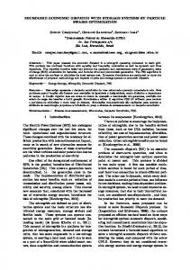
A NUMERICAL EXAMPLE To demonstrate the effectiveness of the MDP model and policy iteration, we apply our approach to a tenbus network example of PJM (Pennsylvania-New Jersey-Maryland Interconnection, 2008), which is a regional transmission organization (RTO) in the eastern United States that operates the world’s largest competitive wholesale electricity market. The network is shown in Figure 1. In this example, all nodes are both demand and supply nodes. Each supply node is assumed to have three generators. Generation and transmission data are given in Tables 1 and 2. Discount rate 𝛽 is set to be 0.95, and system restoration rate is assumed to be 0.0108 (1/hour). Policy iteration is implemented using Matlab (The MathWorks, 2009), Tomlab (Tomlab Optimization, 2009) and Cplex (ILOG Cplex, 2009). The algorithm converges in three iterations within a minute. We compare the optimal MDP policy with the economic dispatch and the N-1 criterion and present the results by answering the following questions.
The initial policy (in Step 1 of policy iteration) is obtained using the economic dispatch for all 𝑠 ∈ {{𝑠𝑁 } ∪ 𝑆𝐶 } × {1,2, . . . ,24}: min
Theorem 1 (Theorem 6.4.6 in Puterman (1994)) The sequence of value vectors {𝑉 𝑖 } generated by policy iteration converges monotonically and in norm to {𝑉𝛽∗ }, which solves the optimality equation (3).
How is the initial policy obtained?
𝑞,𝑑
𝑛∈𝒮
𝑖∈𝐺𝑛
𝑖 𝑏𝑛𝑖 𝑞𝑛,𝑡 +
𝑛∈𝒟
𝑐𝑛LS 𝑑𝑛,𝑡
s.t. 𝑛∈𝒮 𝐻𝑙,𝑛 𝑖∈𝐺𝑛 𝑞𝑛𝑖 ,𝑡 − 𝑛∈𝒟 𝐻𝑙,𝑛 (𝐷𝑛 ,𝑡 − 𝑑𝑛 ,𝑡 ) ≤ 𝑇𝑙 , ∀𝑙 ∈ ℒ, 𝑖 𝑛 ∈𝒮 𝑖∈𝐺𝑛 𝑞𝑛,𝑡 = 𝑛∈𝒟 (𝐷𝑛 ,𝑡 − 𝑑𝑛,𝑡 ),
8
𝑖 0 ≤ 𝑞𝑛,𝑡 ≤ 𝑄𝑛𝑖 , ∀𝑖 ∈ 𝐺𝑛 , 𝑛 ∈ 𝒮; 𝑑𝑛,𝑡 ≥ 0, ∀𝑛 ∈ 𝒟, 𝑡 = 1, . . . ,24.
The objective here is only to minimize the immediate cost, ignoring the risk of future transmission line failures. The policy iteration algorithm starts with this economic dispatch policy and iteratively improves it by balancing the immediate cost and future risk of transmission line failures.
How is the solution to the N-1 criterion obtained?
We obtain the solution to the N-1 criterion for all 𝑠 ∈ {{𝑠𝑁 } ∪ 𝑆𝐶 } × {1,2, . . . ,24} by solving the following problem: min 𝑉 𝑖+1 (𝑠) = 𝑞,𝑑
𝑛∈𝒮
𝑖∈𝐺𝑛
𝑖 𝑏𝑛𝑖 𝑞𝑛,𝑡 +
𝑛∈𝒟
𝑐𝑛LS 𝑑𝑛,𝑡
𝑠 𝑠 𝑖 s.t. 𝑛∈𝒮 𝐻𝑙,𝑛 𝑖∈𝐺𝑛 𝑞𝑛 ,𝑡 − 𝑛∈𝒟 𝐻𝑙,𝑛 (𝐷𝑛 ,𝑡 − 𝑑𝑛 ,𝑡 ) ≤ 𝑇𝑙 , ∀𝑙 ∈ ℒ𝑠 , 𝑘 𝑘 𝑖 𝑛∈𝒮 𝐻𝑙,𝑛 𝑖∈𝐺𝑛 𝑞𝑛,𝑡 − 𝑛∈𝒟 𝐻𝑙,𝑛 (𝐷𝑛,𝑡 − 𝑑𝑛,𝑡 ) ≤ 𝑇𝑙 , ∀𝑙 ∈ ℒ𝑠 \𝑘, ∀𝑘 ∈ 𝑆𝐶 \𝑠,
𝑛∈𝒮
𝑖 𝑞𝑛,𝑡
𝑖∈𝐺𝑛
𝑖 𝑞𝑛,𝑡 =
𝑄𝑛𝑖 , ∀𝑖
0≤ ≤ 𝒟, 𝑡 = 1, . . . ,24.
𝑛∈𝒟
(𝐷𝑛,𝑡 − 𝑑𝑛,𝑡 ),
∈ 𝐺𝑛 , ∀𝑛 ∈ 𝒮; 𝑑𝑛,𝑡 ≥ 0, ∀𝑛 ∈
Here, the dispatch has to satisfies the transmission constraints under not only the current scenario but also all possible scenarios with one more transmission line failure. As such, the N-1 criterion is a more conservative policy than the economic dispatch.
How much improvement does the optimal MDP solution have over the economic dispatch and the N-1 criterion?
We show the differences of economic dispatch, the N-1 criterion, and optimal MDP policy using three measures: immediate costs, stationary state probability distribution, and expected long-term discounted cost. The immediate costs of all states are obtained from the immediate cost vector 𝑐 under the optimal MDP policy. In Table 3, the terms 𝑐𝑠𝑡𝑁 , 𝑐𝑆𝑡𝐶 , and 𝑐𝑠𝑡𝐵 denote the immediate costs at hour 𝑡 under the normal state, an average contingency state, and the blackout state, respectively. For ease of exposition, we will combine the probabilities of all states in the set of contingency states 𝑆𝐶 as one. The stationary state probability distribution is obtained by solving the equation 𝜋 𝛵 𝑃(𝑎 ∗ ) = 𝜋 𝛵 , where 𝑃(𝑎 ∗ ) is the transition probability matrix under the optimal policy 𝑎 ∗ and 𝜋 denotes the stationary probability vector with 𝜋(𝑠) being the stationary probability in
state 𝑠. We will take the average over 24 hours and combine the probabilities of all states in the set of contingency states 𝑆𝐶 as one. The expected long-term discounted costs are obtained from the immediate cost vector 𝑉 under the optimal MDP policy. Here 𝑉(𝑠) is the optimal expected long-term discounted cost if the system starts from state 𝑠, averaged over all 24 hours. Results are given in Table 3. The immediate costs and expected long-term discounted costs are given in $106 , and the stationary state probability distribution has no unit. The immediate costs of all states under all dispatch policies follow a similar temporal pattern with demand fluctuation. Since in a contingency state 𝑠 ∈ 𝑆𝐶 one transmission line is lost but the system is still able to operate using the rest of the lines, the immediate cost is usually slightly higher. However, it is also noticed in several occasions that the immediate cost under a contingency state is smaller than that under the normal state. Although counterintuitive, this is a well-studied effect known as Braess’s paradox. Fisher et al. (2008) and Hedman et al. (2008) have detailed discussions on how removing transmission lines could potentially reduce the generation costs. The economic dispatch has smaller immediate costs than the other two policies under all states and all hours, except the blackout state, in which the dispatch action is interrupted by system restoration and thus all policies have the same immediate cost. The N-1 criterion has the largest immediate costs. The MDP policy’s costs are in between, but closer to the economic dispatch especially under contingency states. Since the economic dispatch minimizes the immediate costs without hedging any risk of transmission line failure, it has the smallest normal state probability 𝜋(𝑠𝑁 ) and highest blackout state probability 𝜋(𝑠𝐵 ). As the opposite, the N-1 criterion hedges every single-contingency in the dispatch decision making, thus has the highest 𝜋(𝑠𝑁 ) and smallest 𝜋(𝑠𝐵 ). The MDP policy is also in between, but closer to the N-1 criterion. The optimal MDP policy is almost as cost efficient as the economic dispatch and almost as secure as the N-1 criterion, therefore, it has the smallest expected long-term discounted costs compared to the other two policies in all states.
CONCLUSION Cost efficiency and security are two main ingredients for an “optimal” dispatch. Cost efficiency means to serve demand with minimum cost, while security requires that electricity be delivered to the customers without interruption even in the event of component
9
failures. In this paper, we have introduced an MDP approach to obtain the optimal balance of these two conflicting objectives for the security constrained economic dispatch problem. This approach quantifies the risk of transmission line failures and minimizes the expected long-term discounted total cost. As an important social service, electric power dispatch is a continuous and uninterrupted process. Many existing models focus on a short period of the process. The MDP approach, on the other hand, allows one to formulate the dispatch process as an infinite horizon problem. Another advantage of the MDP model is its capability to provide not only the optimal preventive actions under the normal scenario but also optimal corrective actions under contingency scenarios. In contrast to standard MDP models, the security constrained economic dispatch problem contains a continuous action space which is defined by generation and transmission constraints. The contribution of this paper also includes using a stochastic programming approach to substitute the policy improvement step of the policy iteration algorithm, since exhaustively enumerating and comparing all feasible actions is no longer a viable strategy. The numerical example of a PJM case study demonstrates the advantage of this model over the economic dispatch and the N-1 criterion. The problem with the economic dispatch is that immediate cost is minimized without consideration of potential risk, whereas the N-1 criterion tends to be over conservative and expensive. Numerical results show that the MDP approach is almost as cost efficient as the economic dispatch, and at the same time achieves a reliability level almost as high as the N-1 criterion. Our MDP model also has some limitations. For example, generator failure and demand uncertainty within a given hour are ignored to reduce the state space and to focus the discussion on the effect of transmission line failures. Future research should integrate generator failure and demand uncertainty with transmission line failure. Computation burden for such an integrated model could be alleviated by heuristic or approximation algorithms.
EFRI-0835989. The second author is supported by Air Force Office of Sponsored Research under Grant FA9550-08-1-0268.
REFERENCES Abrate, G. (2008). Time-of-use pricing and electricity demand response: evidence from a sample of Italian industrial customers. International Journal of Applied Management Science, 1(1), 21-40. Apt, J., Lave, L.B., Talukdar, S., Morgan, M.G., & Ilic., M. (2004). Electrical blackouts: a systemic problem. Issues in Science and Technology, 1-8. Birge, J.R., F.V. Louveaux. (1997). Introduction to stochastic programming. Springer, New York. Bouffard, F., Galiana, F.D., & Conejo, A.J. (2005a). Market-clearing with stochastic security— Part I: formulation. IEEE Transactions on Power Systems, 20(4), 1818-1826. Bouffard, F., Galiana, F.D., & Conejo, A.J. (2005b). Market-clearing with stochastic security— Part II: case studies. IEEE Transactions on Power Systems, 20(4), 1827-1835. Chen, J., Thorp, J.S., & Dobson, I. (2005). Cascading dynamics and mitigation assessment in power system disturbances via a hidden failure model. Electrical Power and Energy Systems, 27(4), 318326. Chen, Q. & McCalley, J.D. (2005). A Cluster distribution as a model for estimating high-orderevent probabilities in power systems. Probability in the Engineering and Informational Sciences, 19, 489505. Chen, Y. & Hobbs, B.F. (2005). An oligopolistic power market model with tradable NOx permits. IEEE Transactions on Power Systems, 20(1), 119129.
ACKNOLWEDGEMENTS
Fisher, E.B., O’Neill, R.P. & Ferris, M.C. (2008). Optimal transmission switching. IEEE Transactions on Power Systems, 23(3), 1346-1355.
The authors gratefully acknowledge the suggestions and advice of Dr. Mainak Mazumdar at the University of Pittsburgh. The authors thank the Editor-in-Chief, Professor John Wang, and three anonymous reviewers for their insightful and constructive comments. The first author is supported by the National Science Foundation under Grant
Harris, K.E. & W.E. Strongman. (2004). A probabilistic method for reliability, economic and generator interconnection transmission planning studies. Power Systems Conference and Exposition, IEEE PES, 1, 486-490.
10
Hedman, K.M., O’Neill, R.P., Fisher, E.B., & Oren, S.S. (2008). Optimal transmission switching — Sensitivity analysis and extensions. IEEE Transactions on Power Systems, 23(3), 1469-1479. Hines, P., Apt, J., Liao, H., & Talukdar., S. (2006). The frequency of large blackouts in the United States electrical transmission system: an empirical study. Techical Report, Carnegie Mellon University. Hines, P. & Talukdar, S. (2006). Controlling cascading failures with cooperative autonomous agents. Technical report, Carnegie Mellon University. Hogan, W.W. (1993). Markets in real electric networks require reactive prices. The Energy Journal, 14(3), 171-200. ILOG Cplex. (2009). Available from http://www.ilog.com.
Stoft, S. (2002). Power system economics. IEEE Press, Piscataway. Talukdar, S., Jia, D., Hines, P., & Krogh, B.H. (2005). Distributed model predictive control for the mitigation of cascading failures. Proceedings of the 44th IEEE Conference on Decision and Control, and the European Control Conference, 4440-4445. The MathWorks. (2009). Available from http://www.mathworks.com. Tomlab Optimization. (2009). Available from http://tomopt.com. Zima, M. & Andersson, G. (2005). On security criteria in power systems operation. Proceedings of the IEEE Power Engineering Society General Meeting, 3, 3089-3093.
NERC. (2002). Disturbances analysis working group database. North American Electric Reliability Council. Available from http://www.nerc.com/~database.html. Overbye, T.J., Cheng, X., & Sun, Y. (2004). A comparison of the AC and DC power flow models for LMP calculations. Proceedings of the 37th Hawaii International Conference on System Sciences. Pennsylvania-New Jersey-Maryland Interconnection. (2008). Available from http://www.pjm.com. PJM Market Monitor. (2007). Available from http://www.pjm.com/markets/marketmonitor/som.html. Puterman, M.L. (1994). Markov decision processes. John Wiley & Sons, Inc., New York. Ragupathi, R. & Das, T.K. (2004). A stochastic game approach for modeling wholesale energy bidding in deregulated power markets. IEEE Transactions On Power Systems, 19(2), 849-856. Schweppe, F.C., Caramanis, M.C., Tabors, R.E., & Bohn, R.E. (1998). Spot pricing of electricity. Kluwer Academics Publishers, Boston. Song, H., Liu, C.C., Lawarrée J., & Dahlgren, R.W. (2000). Optimal electricity supply bidding by Markov decision process. IEEE Transactions on Power Systems, 15(2), 618-624.
11
Figure 1: Schematic of linearized DC network for PJM (map adapted from PJM (2008) with modification)
12
Table 1: Assumed demand and generation data (partially adapted from PJM Market Monitor (2007)) 𝑛 1 2 3 4 5 6 7 8 9 10
𝐷𝑛 3715 3988 4671 1777 2041 2849 4723 2236 1340 5518
𝑏𝑛1 17 10 18 19 17 18 17 14 17 12
𝑏𝑛2 48 60 60 45 44 55 69 50 58 47
𝑏𝑛3 184 125 181 124 193 135 120 125 162 147
𝑄𝑛1 0 1041 1269 472 71 371 2695 0 5 2012
𝑄𝑛2 3545 1676 4423 1681 4083 947 2711 1721 758 3068
𝑄𝑛3 793 523 732 262 515 933 1873 1732 319 1798
𝐷𝑛 is the average of demand at node 𝑛 over 24 hours
Table 2: Assumed transmission data (partially adapted from Chen and Hobbs (2005)) line 1-2 2-3 2-4 4-5 5-3 3-6 3-7 7-6 3-8 8-9 9-10 10-6
reactance 𝑋 (Ω) 0.01550 0.00390 0.01004 0.02814 0.02206 0.01190 0.00197 0.00980 0.00850 0.00190 0.02498 0.00490
thermal limit (MW) 1403 1741 1531 1808 1809 1590 3227 1824 1844 1523 1590 2758
MTTF (hour) 11966 12283 8932 11758 11586 8138 7833 10489 13718 9383 11097 8567
MTTR (hour) 81 24 93 35 20 25 62 47 35 83 59 55
13
hour 𝑡 1 2 3 4 5 6 7 8 9 10 11 12 13 14 15 16 17 18 19 20 21 22 23 24 𝜋(𝑠) 𝑉(𝑠)
Table 3: Comparison of economic dispatch, the N-1 criterion, and optimal MDP policy Economic Dispatch N-1 criterion MDP 𝑐𝑆𝑡𝐶 𝑐𝑆𝑡𝐶 𝑐𝑆𝑡𝐶 𝑐𝑠𝑡𝑁 𝑐𝑠𝑡𝐵 𝑐𝑠𝑡𝑁 𝑐𝑠𝑡𝐵 𝑐𝑠𝑡𝑁 1.131 1.135 28.050 1.155 1.156 28.050 1.155 1.135 1.054 1.059 26.780 1.079 1.079 26.780 1.079 1.059 1.012 1.017 26.076 1.038 1.036 26.076 1.038 1.017 0.994 0.999 25.781 1.021 1.019 25.781 1.021 0.999 1.012 1.017 26.072 1.037 1.036 26.072 1.037 1.017 1.097 1.101 27.492 1.120 1.119 27.492 1.120 1.101 1.250 1.255 30.012 1.278 1.275 30.012 1.278 1.255 1.388 1.394 32.016 1.429 1.429 32.016 1.409 1.394 1.519 1.529 33.333 1.580 1.577 33.333 1.558 1.529 1.643 1.653 34.369 1.706 1.704 34.369 1.684 1.654 1.747 1.756 35.201 1.806 1.807 35.201 1.785 1.756 1.804 1.813 35.660 1.865 1.866 35.660 1.843 1.814 1.829 1.839 35.859 1.895 1.896 35.859 1.874 1.840 1.850 1.861 36.028 1.920 1.921 36.028 1.899 1.861 1.849 1.861 36.021 1.924 1.925 36.021 1.903 1.861 1.859 1.871 36.097 1.939 1.939 36.097 1.917 1.872 1.917 1.931 36.565 2.003 2.003 36.565 1.981 1.931 2.023 2.037 37.379 2.112 2.112 37.379 2.091 2.037 2.028 2.041 37.416 2.115 2.115 37.416 2.093 2.042 1.981 1.995 37.067 2.066 2.066 37.067 2.045 1.995 1.940 1.951 36.744 2.016 2.016 36.744 1.994 1.951 1.778 1.788 35.454 1.843 1.844 35.454 1.822 1.789 1.467 1.479 32.897 1.542 1.541 32.897 1.521 1.479 1.262 1.268 30.181 1.292 1.299 30.181 1.292 1.268 0.923 0.036 0.041 0.939 0.055 0.006 0.937 0.055 35.48 39.86 552.14 32.48 39.56 551.63 32.44 38.94
𝑐𝑠𝑡𝐵 28.050 26.780 26.076 25.781 26.072 27.492 30.012 32.016 33.333 34.369 35.201 35.660 35.859 36.028 36.021 36.097 36.565 37.379 37.416 37.067 36.744 35.454 32.897 30.181 0.008 551.62
14