Evolutionary Optimization An International Journal on the Internet Volume 3, Number 1, 2001, pp.1-26
A Multi-Objective Genetic Algorithm Approach to Feature Selection in Neural and Fuzzy Modeling Research paper Christos EMMANOUILIDIS
[email protected]
School of Computing and Engineering Technology, Informatics Centre, St. Peter's Campus, University of Sunderland, Sunderland, Tyne and Wear,SR6, 0DD, UK
Andrew HUNTER
[email protected]
Dept. of Computer Science, University of Durham, Science Labs, South Road, Durham DH1 3LE
John MACINTYRE
[email protected]
School of Computing and Engineering Technology, Informatics Centre, St. Peter's Campus, University of Sunderland, Sunderland, Tyne and Wear,SR6, 0DD, UK
Chris COX
[email protected]
School of Computing and Engineering Technology, Edinburgh Building, St. Peter's Campus, University of Sunderland, Sunderland, Tyne and Wear,SR6, 0DD, UK Abstract. A large number of techniques, such a neural networks and neurofuzzy systems, are used to produce empirical models based in part or in whole on observed data. A key stage in the modelling process is the selection of features. Irrelevant or noisy features increase the complexity of the modelling problem, may introduce additional costs in gathering unneeded data, and frequently degrade modelling performance. Often it is acceptable to trade off some decrease in performance against a reduction in complexity (number of input features), although we rarely know a priori what an acceptable trade-off is. In this paper, feature selection is posed as a multiobjective optimisation problem, as in the simplest case it involves feature subset size minimisation and performance maximisation. We propose multiobjective genetic algorithms as an effective means of evolving a population of alternative feature subsets with various modelling accuracy/complexity trade-offs, based on the concept of dominance. We discuss methods to reduce the computational costs of the technique, including the use of special forms of neural network and neurofuzzy models. The major contributions of this paper are: the formulation of feature selection as a multiobjective optimisation problem; the use of multiobjective evolutionary algorithms, based on the concept of dominance, for multiobjective feature subset selection; and the application of the multiobjective genetic algorithm feature selection on a number of neural and fuzzy models together with fast subset evaluation techniques. By considering both neural networks and neurofuzzy models, we show that our approach can be generically applied to different modelling techniques. The proposed method is applied on two small and high dimensional regression problems. Keywords: Multi-objective evolutionary algorithms, Feature Selection, Neurofuzzy modelling, Neural Networks
1. Introduction Feature selection is the process of selecting a subset of available features to use in empirical modelling. Although usually conceived of only as a pre-processing stage, it actually involves model building in order to evaluate proposed feature subsets. The solution to the
2
A Multi-Objective Genetic Algorithm Approach to Feature Selection …
feature selection problem is neither trivial, nor unique. The set of optimal features can be different for different hypothesis spaces. Therefore, optimality of a feature set should only be defined in the context of the family of admissible modelling functions from which it is intended to select the one that is finally deployed (Kohavi and John 1997). It is, for example, of limited value to select input features using a linear model, and then to perform the final modelling with a non-linear model. A desirable property of feature evaluation rules is monotonicity, i.e. addition of features cannot cause performance degradation. Unfortunately, this cannot always be guaranteed in empirical modelling, as adding features may in some cases lead to error rate deterioration (Raudys and Jain 1991; Trunk 1979). Such difficulties imply that even for a fixed family of admissible functions, optimal feature selection can only be guaranteed by exhaustive search of all possible feature subsets. However, exhaustive evaluation is clearly impractical when the problem involves a significant number of features. The process is further complicated by the fact that features are rarely independent. Features with good predictive performance might be sensibly omitted because the model uses other variables that carry the same information - the problem of variable redundancy. There may also be subsets of variables that, when included together, convey important information but individually convey none - variable interdependency. Furthermore, relevant features may well have to be excluded from the optimal subset, while irrelevant features may have to be included in it. Such subtleties are often overlooked when feature selection is based on simple correlation tests, or on information measures such as mutual information, between the potential predictors and the output variable. When the estimated error rate is employed to evaluate feature subsets, there is little benefit in evaluating features individually, as what actually matters is how groups of features perform together. Feature search methods based on generating a single solution, such as the popular forward stepwise approach, can fail to select features which do poorly alone but offer valuable information together (Berk 1978). Branch and bound methods can guarantee an optimal solution, assuming that the feature evaluation criterion is monotonic, i.e. adding features cannot decrease performance (Narendra and Fukunaga 1977). However, error rate estimation based on limited sample sizes cannot guarantee monotonicity, which may for example result in cases where the best subset of features might not even contain the single best individual feature (Toussaint 1971). It is worth noting that such scenarios are possible even in the case of conditionally independent features. The extent to which such anomalous orderings of feature subsets can occur is surprisingly wide (Cover and Campenhout 1977). For such reasons, even the more flexible generalised stepwise and floating search methods (Kittler 1978; Pudil et al. 1994) may have difficulties in cases of highly non-nested feature subsets, although they offer substantial improvements in terms of search flexibility at the expense of increased computational costs compared to stepwise methods (Jain and Zongker 1997). Approaches that maintain a population of solutions, such as genetic algorithms can perform efficient searches in high dimensional spaces with strong interdependencies among the features, while being flexible in the way they explore the search space, compared to greedy hill-climbing methods (Siedlecki and Sklansky 1989). In this paper it is argued that the feature selection problem can naturally be posed as a multiobjective problem, since in the simplest case it involves subset size minimisation and performance maximisation. However, in multiobjective problems there is rarely a single optimal solution but instead we deal with a set of non-dominated solutions, based on the concept of Pareto optimality. This work proposes the use of multiobjective GAs for feature selection. To demonstrate that the feature selection approach is generic, we apply it to three
C. Emmanouilidis, A. Hunter, J. MacIntyre, C. COX
3
different modelling approaches: two forms of neural networks, and neurofuzzy modelling. The developed methodology is simple, and can be applied to real world problems of significant dimensionality. There is a clear lack of work in the literature on search methods for multiobjective feature selection, since the problem is usually treated as a singleobjective one. This makes difficult a direct comparison with existing methods. We test the technique on two real world problems of small and high dimensionality. On the smaller dimensionality set we compared the performance of the multiobective feature selection approach against the stringent test of exhaustive evaluation. Neural networks are widely used in empirical modelling. They have powerful nonlinear modelling capabilities, and require little domain knowledge to be applied. Yet, inclusion of many irrelevant or noisy features can unnecessarily complicate the modelling process. In addition, it is often useful in practical situations to be able to assess the impact of different subsets of inputs on the modelling performance, since such information can guide decisions related to data acquisition and costs and difficulties associated with it. Fuzzy set methods are popular modelling approaches, allowing the user to combine domain knowledge with learning capabilities. Fuzzy systems are particularly widely used in Engineering problem domains (Mendel 1995). Fuzzy systems process both numerical data and linguistic information. An attractive feature of fuzzy modelling is that it can be based on either domain expert knowledge or on sample data or even on both. However, building fuzzy models from data can be problematic in high dimensional spaces. In such cases, feature selection is of critical importance. Despite the weakness of many fuzzy modelling approaches in high dimensional input spaces, the problem of feature selection for fuzzy modelling has not yet attracted enough attention. The major contributions of the paper are: posing feature selection as a multiobjective search problem; the use of multiobjective GAs in the feature selection problem; and the application of the multiobjective GA feature selection on three neural and fuzzy families of models in a way that allows fast feature subset evaluation. Even though genetic algorithms have been used in the past for feature selection, the use of multi-objective algorithms based on the concept of dominance is novel in this application. The structure of the paper is as follows. Sections two and three discuss the application of genetic algorithms to feature selection. In particular, section three poses feature selection as a multiobjective search problem and explains in detail the GA approach taken in this work. Section four discusses the key issue of efficient evaluation of feature subsets selected by the GA. Section five gives the results of our experiments with the technique. Section six is the conclusion.
2. Genetic Algorithms for Feature Selection Genetic algorithms are a natural approach for performing subset selection. A feature subset is represented as a bit-string, with the setting of each bit indicating whether the corresponding feature is used, or not. Feature selection problems are often complicated by interactions between subsets of interdependent or mutually redundant variables, and the hope is that a Genetic Algorithm should be able to exploit epistatic interactions between the bits. Yet, even for single objective problems, GAs can prematurely converge to sub-optimal solutions. This can be due to the existence of super-fit individuals, which dominate the entire population at an early stage. Many modifications of the basic GA have been proposed and implemented, which balance population diversity with selective pressure (Goldberg 1989; Hunter 1998).
A Multi-Objective Genetic Algorithm Approach to Feature Selection …
4
Feature selection algorithms are often classified as “wrapper” and filter approaches (Kohavi and John 1997), while feature weighting methods are also considered (Blum and Langley 1997). The simplest approach to evaluation of a subset of features is to build a model of the same type and complexity as it is intended to ultimately deploy; this is known as the wrapper approach (Kohavi and John 1997). However, the wrapper approach involves high computational costs, as it requires model building for each fitness assignment. Previous work using GAs for feature selection includes feature evaluation with k-Nearest Neighbours (e.g. (Siedlecki and Sklansky 1989)), Multilayer Perceptrons (e.g. (Peck and Dhawan 1996)), Radial Basis Functions , RBFs (Billings and Zheng 1995), Linear Models (e.g. (Broadhurst et al. 1997)), Decision Trees (e.g. (Bala et al. 1995)), Decision Tables (e.g. (Guerra Salcedo et al. 1999)), Probabilistic Neural Networks (e.g. (Hunter 2000)), Naïve-Bayes (e.g. (Inza et al. 2000)), Fuzzy Models (e.g. (Emmanouilidis et al. 1999)), Counter Propagation Networks (e.g. (Brill et al. 1992)), Partial Least Squares (e.g. (Leardi and Gonzalez 1998)), as well as with indirect feature evaluation criteria, such as Mahalanobis distance (e.g. (Jain and Zongker 1997)) and Mutual Information (e.g. (Weiquan et al. 1995)). The major computational cost when using GAs for “wrapper” feature selection is in the feature subset evaluation. This requires building a computational model using the selected subset of input variables, followed by evaluating the model's performance, typically by testing against a hold-out set. Depending on the complexity of the modelling problem, this can make the whole procedure computationally prohibitive. Genetic Algorithm feature selection can also be performed using a “filter” approach, i.e. by completely separating the feature selection stage from the modelling stage (Liu et al. 1995). “Filter” approaches, though computationally attractive, are less reliable than “wrapper” ones. In this paper we steer a middle course between wrapper and filter approaches. Subset evaluation is performed in the same hypothesis space, and with the same model induction algorithm, as is intended for the final stage of modelling. However, we take advantage of approaches that allow the use of a fast fitness evaluation procedure.
3. Multiobjective GA Approach for Feature Selection Feature selection involves a two stage-optimisation procedure: the first stage is a combinatorial optimisation problem, which involves searching in a search space of 2 M − 1 solutions; the second stage is the subset evaluation and can be considered as a standard optimisation problem, which primarily depends on: •
The hypothesis space, H, i.e. the family of admissible functions which from the one that is finally deployed is drawn.
•
The feature evaluation criterion, e.g. the estimated error rate.
•
The data availability.
Subset evaluation further depends on the actual induction algorithm employed in order to build the empirical model. Clearly, identifying a solution to the combinatorial search problem presupposes that the second-stage problem, that of feature evaluation, is also tackled, if the wrapper approach is to be employed. The performance of the induced model and the subset cardinality jointly offer a measure of the quality of the solution. If a fixed hypothesis space and induction algorithm are assumed, then the feature selection problem for a given hypothesis space H is to select a subset S j so that:
C. Emmanouilidis, A. Hunter, J. MacIntyre, C. COX
5
S j ( H (x)) = arg min{J (x)} (1) j S ∈S where the objective function J(x) is a vector consisting of at least two terms: the first one is the subset cardinality, S j ; and the second is a performance measure, which in the simplest case is the misclassification rate in classification, or an error norm, such as the L1 or L2 norms, in regression. Additional performance objectives may also be included, such as the true positive and true negative classification rates or misclassification and data acquisition costs. Typically, in multiobjective optimisation problems there is no single optimal solution, but a range of Pareto optimal solutions. The key concept here is dominance: Dominance Relation: A solution J1 is said to dominate a solution J2 (written as J1 pJ 2 ) if and only if the following two conditions hold at the same time: •
J1 is no worse than J2 in any of the objectives.
•
J1 is strictly better than J2 in at least one objective
A solution is said to be Pareto optimal if it cannot be dominated by any other solution available in the search space. Whereas in single-objective optimisation solutions can be ordered, depending on the optimisation criterion value they achieve, in multi-objective optimisation such simple ordering does not generally exist. As the objective function in feature selection is at least two-dimensional (i.e. consisting of a complexity and a performance term in the simplest case), the solution need not be a single one, but instead a range of non-dominated solutions. There are many reasons why it is desirable to discover such a set of Pareto optimal solutions in feature selection. Weighting coefficients. Feature selection often aims to discover a single solution by means of optimising a composite cost function, which weights the performance and complexity terms. This scalarisation of a set of objectives into a single objective presents a clear problem, that of how to choose the weighting coefficients. Setting aside obvious scaling problems (the two objectives usually lie in different ranges, therefore some objectives normalisation is usually deemed appropriate), depending on the exact choice of the weighting coefficients, different solutions may be found. However, there is usually little or no prior knowledge with respect to the modelling problem – this is one of the reasons why there is a need for feature selection – and therefore it is not at all clear what constitutes a good choice of such coefficients. Selection bias and trade-offs. An extreme case is when the weighting coefficient for complexity is zero. Essentially this implies that the aim is to identify the feature subset which achieves maximum performance. When the performance measure is the error rate, the fundamental problem lies with the reliable estimation of this rate. This is usually achieved by means of cross-validation, which reduces the bias or variance or indeed both bias and variance of the error rate estimates but does not bring it down to zero. If the error rate is the only criterion, then even the tiniest of improvements in it, which may well be attributed to data or modelling noise, will lead the feature selection procedure to select subsets of higher complexity. In the absence of a set of non-dominated solutions, it is not at all clear what is the significance of adding such a number of superfluous features. In contrast, when such a set of solutions is available, a user can identify the trade-off that appears to be appropriate for the particular modelling problem. It is worth noting that such
6
A Multi-Objective Genetic Algorithm Approach to Feature Selection …
a choice is made a-posteriori and therefore does not influence the outcome of the feature selection. Additional objectives. The obvious choice for assessing a classifier’s performance is to estimate its misclassification rate. However, in many problem domains, such as in engineering or medical diagnosis, it makes more sense to optimise alternative objectives, such as the specificity and sensitivity of a diagnostic model, as well as misclassification and data-acquisition costs. The ability to discover a range of solutions with different objectives trade-offs can facilitate more informed choices with regard to laboratory tests, or data acquisition and processing. Obtaining such non-dominated solutions to the subset selection problem would be difficult for a conventional single-objective algorithm, yet it is a natural outcome for a Pareto-based feature selection approach. Although in this paper we focus on experimentation with two objectives, the multiobjective GA feature selection approach can be extended to handle such additional objectives. It is frequently useful to select not just a single feature subset, but a range of subsets with different trade-offs between performance and complexity (i.e. we may tolerate lower performance in a model that also requires less features). Since the GA is population based, it seems natural to look for a method that produces a diverse range of such feature sets in the final population. This also helps to mitigate the problem of premature convergence, to which GAs are prone. We therefore use a multiobjective GA, where there are two objectives: to minimise the number of features in the subset, and to maximise modelling performance. Although the feature selection problem is well-suited for multiobjective optimisation, in the literature it is usually considered as a single-objective optimisation problem. A common choice for a multiobjective GA is to aggregate the different objectives by introducing a single, composite objective function (Yang and Honavar 1998). The main drawback of such an approach is that it makes it very difficult to explore different possibilities of trade-offs between model accuracy and complexity, as it biases the search towards a pre-determined trade-off. Single objective GAs could also be used to optimise performance for a given subset size. This can be pursued in a number of ways but, in principle, it would involve evolving a population of solutions increasingly concentrated around the desired subset size. Such an approach would limit the possibility for creative recombination of the genetic material between individuals whose complexity differs from the desired one. However, a significant part of the exploratory power of a genetic algorithm is attributed to the recombination operator and its ability to discover good solutions by building on existing schemata of promising performance. By imposing restrictions on the subset size, there is a danger of eliminating useful population diversity. Thus, chromosomes of diverse subset size may not stand a chance to pass on well performing schemata to the next generation. Such population diversity is more likely to be maintained by aiming both at subset size minimisation and performance maximisation, without specifying which objective is more important. We therefore treat feature selection as a multiobjective optimisation problem, in the Pareto sense. The absence of work on multiobjective feature selection is reflected also in the lack of algorithmic implementations for multiobjective feature search. Part of the problem lies with the sheer complexity of the search task. The search space becomes huge, even for moderately sized feature subsets. Therefore, in most applications a non-exhaustive algorithm is employed to find a near optimal feature subset. However, in the case of multiobjective optimisation the very notion of a single optimal solution collapses. A search algorithm is not only faced with the – already difficult – task of discovering a single, near-
C. Emmanouilidis, A. Hunter, J. MacIntyre, C. COX
7
optimal solution, but with the more complicated problem of finding a set of non-dominated solutions. This paper explores the possibility of applying multiobjective Genetic Algorithms for feature selection. Such algorithms are rapidly emerging as a viable alternative in complex multi-objective search and optimisation problems (Deb 2001). It is worth noting that the different nature of single-objective and multi-objective problems makes it difficult to perform a direct comparison between single-objective and multiobjective search algorithms. The first multiobjective GAs was Schaffer’s Vector Evaluated Genetic Algorithm (VEGA) (Schaffer 1985). VEGA develops a population of solutions by splitting it at each generation to different sub-populations, each one of them assigning fitness to its members based on a different objective. The mating pool is then formed by shuffling the individuals selected from each sub-population. However, this method produces mostly solutions that perform well for each objective separately, thus some of the diversity of the actual nondominated solutions is often missed (Deb 2001). Since Schaffer’s early work, several different multiobjective evolutionary algorithms have been implemented, based on the concept of dominance and aimed at approximating the Pareto optimal set of solutions. Surveys of such implementations can be found in (Deb 2001) (Coello 1999) (vanVeldhuizen and Lamont 2000). We employ a variation of the niched Pareto GA (NPGA) (Horn 1997; Horn et al. 1994). This is known to be a fast MOEA (Coello 1999) since tournament domination is determined by a random sub-sample of the population. However, any MOEA could be employed in this setting. Niching techniques can maintain population diversity by employing techniques such as fitness sharing (Goldberg 1989). The NPGA algorithm uses a specialised tournament selection approach, based on the concept of dominance. The common choice is to hold binary tournaments, although selection pressure can be increased by holding tournaments with more than two candidates. The selection procedure is as follows: 1. Individuals are randomly selected from the population to form a dominance tournament group. 2. A dominance tournament sampling set is formed by randomly selecting individuals from the population. 3. Each individual in the tournament group is checked for domination by the dominance sampling group (i.e. if dominated by at least one individual). 3a. If all but one of the individuals in the tournament group are dominated by the dominance tournament sampling group, the non-dominated one is copied and included in the mating pool. 3b. If all individuals in the tournament group are dominated then they are all considered for selection. 3c. If at least two of them are non-dominated, the non-dominated ones are considered for selection. 3d. In the last two cases the individual with the smallest niche count is selected, as this maintains diversity. The niche count for each individual is calculated by following a typical sharing technique: d ij s (dij ) = 1 − σ S 0
αs
if otherwise
dij < σ s
(2)
8
A Multi-Objective Genetic Algorithm Approach to Feature Selection … mi = ∑ s(d ij ) N
(3)
j =1
where mi is the niche count of the i-th individual in the tournament group, s is calculated by the Hamming distances d ij of the above individual with each of the N individuals already present in the mating pool and σ s is the Hamming distance threshold, below which two individuals are considered similar enough to affect the niche count and α s is often set to one to correspond to triangular sharing function. 4. If the mating pool is full, end tournament selection; otherwise go back to step 1. Using some simple bitwise functions, Schaffer’s F2 function (Schaffer 1985), and a real world problem of larger size, (Horn 1997) reported that this random sampling dominance tournament selection was superior to a simple dominance tournament, where the winner was chosen by checking for dominance within the tournament group. Using Horn’s approach, the domination pressure can be controlled by appropriate choice of the size of the dominance tournament sampling set and the niching parameters. In the experiments with the unbalance data set, which involves a large number features we observed a strong tendency of over-sampling medium sized subsets. This is primarily attributed to the standard crossover operator, which tends to average the selected bits of the mating partners. There we found it more appropriate to employ a composite distance function as follows: d ij = d ijh + d ijc 2
2
(4)
where d ij is the Euclidean distance of the above individual to the jth of the N individuals already present in the mating pool, d ijh and d ijc are the corresponding distances in the Hamming and complexity space respectively. This niching technique allows the selection of dissimilar subsets that may achieve good performance at the same complexity level, while preventing domination of the population by a single very fit individual at early stages of the process. It also balances the population distribution across the subset size space. Hence, it enables more exploration to take place across a wider range of the non-dominated front, counter-balancing to some extent the tendency of the crossover operator to produce medium-sized subsets. This paper proposes the use of multiobjective evolutionary algorithms for feature selection and demonstrates the efficacy of such a multiobjective genetic algorithm on the extremely challenging feature selection problem.
4. Efficiency of Feature Subset Evaluation The major computational cost associated with the use of GAs for feature selection is in the evaluation of the feature subsets. Typically, this involves building and evaluating a proposed model using a given feature subset. In order to avoid the computational costs associated with the wrapper approach, one can use a simpler form of model that can be evaluated more quickly during the feature selection stage. We distinguish two methods to reduce the computational cost involved in the evaluation of the feature subsets. First, one can choose a method that, although related to the form of model intended, is simplified or constrained in some fashion. For example, one could
C. Emmanouilidis, A. Hunter, J. MacIntyre, C. COX
9
choose neural networks with a limited number of weights, or trained for a limited period of time. We use a radical form of this procedure, deploying a particular form of neural network (probabilistic and generalized regression neural networks, PNNs and GRNNs) which have particularly low training requirements, but have performance comparable with other forms of neural networks. We may use these even if we ultimately intend to deploy a different form of neural network. In this approach, we risk moving relatively far from the target hypothesis space. However, we do know that GRNNs and PNNs are, like other forms of neural network, non-linear, and usually have comparable performance. They are also very closely related to Radial Basis Function networks, so this risk is justified. Second, one can select a form of model such that a master model can be optimised at the beginning of the feature selection process. The master model uses the entire variable set, but can be deployed in such a way that unavailable features can be eliminated from consideration during feature subset evaluation, without requiring retraining of the master model. As the master model is optimised only once, we can afford to use advanced and time-consuming optimisation strategies. We demonstrate how the master model approach can be deployed both with neurofuzzy and with neural network models. 4.1 Evaluation on Generalized Regression Neural Networks Generalized Regression Neural Networks (Specht 1991) and Probabilistic Neural Networks (Specht 1990) are suitable for feature selection as they are very fast evaluating neural network techniques. They estimate the output from a new pattern using the combination of (typically Gaussian) kernel functions located at each training case. The GRNN is used for regression problems, and the PNN for classification problems. The GRNN estimates the regression output as: ∞
E[ z x] =
∫ zf (x, z)dz
−∞ ∞
(5)
∫ f (x, z )dz
−∞
z is the output value, which is being estimated; x is the input (test) case; f is the joint probability density function of the inputs and outputs. As the joint probability density function is not known, it is estimated using a sum of Gaussian kernel functions located at each pattern in the training data set. To evaluate a feature subset, we split the available data into training and verification patterns. A hold-out set is kept for final evaluation. We then accumulate the root mean squared residual error when estimating each verification pattern output using the training patterns. The execution time of the GRNN (there is, in effect, no training time) is proportional to ( N t N v M s ) , where Nt and Nv are the number of training and validation patterns respectively and Ms is the number of variables in the subset. During the evolutionary process, Ms can be approximated by M/2 over the whole population, where M is the total number of available variables. Considering that the number of training and validation patterns is a fraction of the total number of patterns, N, the cost of feature evaluation with GRNNs is a fraction of MN2. This compares favourably with iterative algorithms such as Back Propagation, which have training times typically proportional to at
10
A Multi-Objective Genetic Algorithm Approach to Feature Selection …
least M2N (and perhaps to higher powers of M), but with a constant of proportionality very high due to the large number of iterations that must be undertaken during training. Nonetheless, it can be seen that the complexity of GRNN feature evaluation grows considerably for data sets involving large number of samples, though it is extremely efficient for data sets of up to approximately 2,000 patterns. In larger data sets it is possible to sub-sample. The stochastic nature of the GA makes this more acceptable than in algorithms that never retest the same feature subsets. 4.2 Neural Networks as Master Models A second possible approach is to employ a standard neural network model as a master model. A neural network is trained using the full range of available input features before the feature selection algorithm begins. Any form of neural network can be used in this approach. To evaluate a feature subset, we wish to "eliminate" unavailable features from this model. We could achieve this in two ways: 1. Delete the input neurons corresponding to the eliminated features; 2. Feed information to the neural network as if the eliminated features were "unknown". The first approach can be simulated by feeding a zero into the "eliminated" input in place of the actual feature value, and has been suggested before (De et al. 1997). However, the approach leads to bias, as the hidden layer thresholds are adjusted during training in part to reflect the average input to the eliminated input. We have adopted a more viable approach, based upon tackling the missing value problem. In many real world problem domains the values of input variables may be missing. We seek a method that allows us to continue to deploy a predictive model even in the absence of some information. There are a variety of possible approaches. The simplest is to substitute the sample mean of the feature from the training set. More complex approaches, such as data imputation (where auxiliary models are used to estimate the missing variable based on the value of other, known, inputs) could also be used. However, we employ sample mean substitution. For feature selection, we first train a master model to accept all input variables. To evaluate a feature subset, we test the master network on the test data. Features that are selected in the feature mask are copied from the data set. Features that are not selected in the feature mask, instead have the sample mean value provided. The deterioration in model performance indicates the efficacy of the feature subset. Multilayer perceptron training in this work is done with the Quasi-Newton method (BFGS) using the Trajan Neural Network Software (www.trajansoftware.demon.co.uk/commerce.htm). 4.3 Evaluation on Neurofuzzy Models Among the different approaches to intelligent computation, fuzzy logic provides a strong framework for achieving robust and yet simple solutions. A large number of adaptive fuzzy or neurofuzzy models have been reported in the literature, which aim at amalgamating the benefits of both computational approaches, namely the learning capabilities of neural networks and the representation power and transparency of fuzzy logic systems. When building neurofuzzy systems for a non-trivial problem, there is usually a trade-off between model interpretability and performance. This is reflected in the two different approaches currently available in neurofuzzy computing. The first one is focused on building functional
C. Emmanouilidis, A. Hunter, J. MacIntyre, C. COX
11
fuzzy models. These are in essence weighted local models. The second approach aims to build fully transparent fuzzy systems, having fuzzy output sets as consequent parts of the fuzzy rules. The former gives better approximations, but as the dimension of the problem increases, model transparency is sacrificed. The latter preserve model interpretability but the complexity is transferred to the size of the fuzzy rule base. Layer 1
x Layer 2
Layer 3
Layer 4
A11 w1
Ð1
A1j
N1
w1N
f1(w1N,x)
A1L
x
.. .
.. .
.. .
x1
.. .
Layer 5
Ai1
.. .
Aij
xi .. .
AiL
xL
.. .
wi
Ðj
Nj
.. .
wjN
y fj(wjN,x)
Ó
.. .
.. .
An1 wL
ÐL
Anj
NL
wLN
fL(wLN,x)
AnL
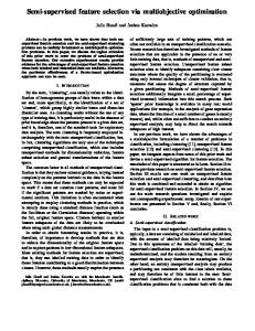
Figure 1. ANFIS architecture
We focus on functional fuzzy models - in particular on fuzzy models having zero or first order polynomials as consequent parts. These are also known as Adaptive Network-Based Fuzzy Inference Systems (ANFIS) (Jang 1993). A typical diagram showing the functionality of an ANFIS model is shown in Figure 1. The input output mapping performed by an ANFIS model is: L
L
y=
n
∏ µ A ( xi ) ⋅ f j (x ) ∑ w j ⋅ f j ( x) ∑ j =1 i =1 j =1
L
wj ∑ j= 1
=
ij
L
(6)
n
µ A ( xi ) ∑∏ j= 1 i =1
ij
where L is the number of the fuzzy rules, µ Aij ( xi ) is the degree (membership value) to which the input xi satisfies the premise part of the j-th rule, n is the dimension of the input vector, y is the network output and f j (x ) is the consequent function of the j-th rule. We employ a method for constructing ANFIS models based on cluster estimation out of data, called subtractive clustering (Chiu 1994). A key characteristic of this model is that it is straightforward to study the effect of removing an input, by simply removing all the antecedent clauses in Equation 6 which are associated with the deleted input. We can thus deploy the model for feature selection as a master model. Following such an approach, Chiu (Chiu 1994) developed a backwards elimination procedure to perform input selection. The basic idea is to build an initial 0-order ANFIS model (i.e. a model with singleton consequent parts) and study the effect of input removals on that. The premise parts of the initial ANFIS model are identified by cluster estimation, whereas the optimal consequent parts for the current premise parameters are optimised
12
A Multi-Objective Genetic Algorithm Approach to Feature Selection …
using linear least squares. Fine-tuning of both the premise and consequent parameters is performed by a gradient descent algorithm. Usually, a small number of iterations are needed, since the initial model is already a fairly good one. It is argued that as long as the initial fuzzy model does not overfit the data, such an evaluation is a reliable way of estimating the influence of each variable on the output (Chiu 1994). Although such an approach cannot be as accurate as a full wrapper evaluation, it is adopted here to circumvent the high computational costs involved with full model construction for each subset evaluation. We have extended Chiu's work by using the multiobjective GA described in the previous section to search for Pareto-optimal subsets of inputs. Here, we also find it practical to let the subtractive clustering algorithm choose large and well-defined clusters, with their radius of influence across each input dimension determined by the standard deviation of the available training data on this dimension. Thus, the clusters' shape is tailored to better represent the input/output association of the data. The subtractive clustering algorithm belongs to a family of algorithms based on computing action potentials, such as the mountain clustering algorithm (Yager and Filev 1994). When determining the action potentials, which in turn determine the location of the clusters, the input/output association is also taken into account. We always employ a much smaller range of influence for the output dimension, so that the identified clusters represent inputoutput relationships, rather than groupings of data simply in the input space. The input/output relationship of fuzzy systems can be expressed as a fuzzy basis function (FBF) expansion (Mendel 1995), similar to equation (3). The relationships between FBFs and other basis functions have been studied in (Hunt et al. 1996; Kim and Mendel 1995) Neural networks with one hidden layer can also be expressed as a basis function expansion of similar form. As a result of such comparisons, the functional equivalence between certain classes of fuzzy inference systems and neural networks has been established (Hunt et al. 1996; Jang and Sun 1993). This equivalence applies mainly to neural networks with local receptive fields, such as those employing Gaussian or B-spline basis functions.
5. Results and Discussion The multiobjective genetic algorithm approach to feature selection was tested on the following two data sets: Rotating Machinery Fault Diagnosis based on vibration data. The data set consists of 3068 patterns randomly split into training, verification and final independent test sets of 1534, 767 and 767 patterns respectively. The algorithm has to choose out of 56 spectral and cepstral features (cepstrum is an anagram of spectrum and stands for the spectrum of the logarithm of the power spectrum of the vibration signal). The output is the estimate of unbalance fault severity, quantified on a scale between 0-100, where 0 corresponds to absence of the specific fault and 100 to the presence of a severe fault (Jantunen and VähäPietilä 1997). The data correspond to various scenarios, including healthy, single fault and multiple fault cases, in the presence of noise. Among the potential predictor variables there is considerable information redundancy and strong interdependencies or correlation among some of them. Exhaustive search in this data set would involve 7,2058e+16 evaluations. Building Energy Consumption Prediction. This is a standard benchmark problem, which involves predicting the hourly consumption of electrical energy in a building, based on the
C. Emmanouilidis, A. Hunter, J. MacIntyre, C. COX
13
date, time of day, outside temperature and air humidity, solar radiation and wind speed. It is taken from “The Great Energy Prediction Shootout – the first building data analysis and prediction problem"” a contest organised in 1993 for the ASHRAE Meeting in Denver, Colorado, USA. The data is employed in exactly the same form as in the PROBEN1 benchmarking problems database (Prechelt 1994). The data consists of 4208 patterns, split into 2104, 1052 and 1052 data sets for training, verification and final independent test respectively. Most predictor variables convey some useful information for modelling. Exhaustive search of subset requires 16383 evaluations. 5.1 Fault Diagnosis in Rotating Machinery A series of experiments have been conducted, in order to study the impact of modifying various algorithmic parameters to the effectiveness of the input selection procedure. The following GA settings were applied: mutation rate: 0.03; 2 point crossover; elitism (the individual with the best performance is copied to the next generation); tournament size 2; Four multiobjective GA runs were executed for each model, i.e. Fuzzy, MLP and GRNN, in order to study the ability of the algorithm to discover sets of non-dominated solutions. Initial experiments were contacted with a population size of 100. However, due to the scale of the problem, involving 56 features and non-dominated fronts of more than 30 solutions, a population of 250 seemed more appropriate. The experiments involved 250 generations, apart from the fuzzy model feature selection, which involved smaller non-dominated fronts and populations of 200 individuals were evolved for 200 generations. The tournament sampling set size was set to one tenth of the population size (Horn 1997). Two crossover rates were employed, 0.4 and 0.8; however, no significant variation in the obtained results was observed.
25
RMSE
20 15 10 5 0 0
0 20
20
40 60
40 80 100
60
Subset Size
Generations
Figure 2. Multiobjective GA progress in 100 generations (Fuzzy Model)
A Multi-Objective Genetic Algorithm Approach to Feature Selection …
14
Input Selection for Fuzzy Models. The GA solutions are evaluated based on simple 0order ANFIS models. Once the influential inputs are identified, one can choose between building either 0-order 1st-order ANFIS models. The first ones are more appropriate when model transparency is a critical issue. The latter can more efficiently capture functional dependencies, which can be modelled by building locally weighted approximations. Four runs with different random intitialisations were performed to study the ability of the algorithm to discover feature subsets across the range of the non-dominated front. A snapshot of the population at one of the GA runs for each generation is shown in Figure 2, where the root mean squared error of the best individual at each complexity level and at each generation is illustrated. This is based on an initial 0-order model with 10 fuzzy rules. It is worth noting that the initial fuzzy model is not a very accurate one. We trade-off some accuracy to achieve faster fitness evaluation. Keeping the initial models small and compact reduces the chances of overfit and consequently increases the chances that any selected input has a true contribution to the modelling performance and its selection is not a result of noise originating from overfit (Chiu 1994). The best individuals over the entire evolution process at each generation are shown in Figure 3. The non-dominated individuals at each complexity level over the entire evolution process are shown in Figure 4. The best individuals at each complexity level are marked by a cross. When they also belong to the non-dominated set they are also circled. The non-dominated set for the unbalance problem implies the set of non-dominated solutions found over all the experiments performed, while in the smaller dataset of building energy prediction it implies the true set of Pareto optimal solutions, identified by exhaustive evaluation.
20
RMSE
15 10 5 0 0
0 20
20
40 60
40 80 100
60
Subset Size
Generations
Figure 3. Best Individuals During Evolution (Fuzzy Model)
C. Emmanouilidis, A. Hunter, J. MacIntyre, C. COX
15
16 15.5 15 14.5
RMSE
14 13.5 13 12.5 12 11.5 11
0
5
10
15
Subset Size
Figure 4. Non-dominated individuals after four multiobjective GA runs (Fuzzy Model)
Input Selection for Multilayer Perceptrons. Four multiobjective GA experiments were also contacted for MLP feature selection, based on a 1-hidden layer multilayer perceptron with sigmoid activations and 14 hidden units. The difference with the fuzzy model feature selection was that the size of the evolved non-dominated frontiers was larger. The nondominated individuals at each complexity level and at each generation in one of the GA runs are shown in Figure 5. In Figure 6, the non-dominated individuals among all those explored are shown. Finally, Figure 7 illustrates the non-dominated individuals over the entire evolution process, based on the master multilayer perceptron model.
25
RMSE
20 15 10 5 0 0
0 20
20
40 60
40
80 100
60
Subset Size
Generations
Figure 5. Multiobjective GA progress in 100 generations (MLP)
16
A Multi-Objective Genetic Algorithm Approach to Feature Selection …
25
RMSE
20 15 10 5 0 0
0 20
20
40 60
40 80 100
60
Subset Size
Generations
Figure 6. Best Individuals During Evolution (MLP) 22 20 18
RMSE
16 14 12 10 8 6 4
0
10
20
30 Subset Size
40
50
60
Figure 7. Non-dominated individuals after four multiobjective GA runs (MLP)
Input Selection for General Regression Neural Networks. In the case of general regression neural networks (GRNN), the one-pass training involved permits instantaneous model building for each individual of the population at each generation, i.e. a full wrapper method. The critical parameter in this case is the smoothing factor. Since the training of GRNNs is trivial, the identification of the appropriate smoothing factor is easily done by experimentation. Here, a smoothing factor of 0.3 is employed. The best individuals at each
C. Emmanouilidis, A. Hunter, J. MacIntyre, C. COX
17
generation, over 100 generations of one multiobjective GRNN feature selection experiment are shown in Figure 8. The non-dominated individuals found so far at each generation are shown in Figure 9. In Figure 10 the best individuals at each complexity level as derived from the four multiobjective GA feature selection experiments are shown.
0.2
RMSE
0.15 0.1 0.05 0 0
0 20
20
40 60
40 80 100
60
Subset Size
Generations
Figure 8. Multiobjective GA Progress in 100 generations (GRNN)
0.2
RMSE
0.15 0.1 0.05 0 0
0 20
20
40 60
40 80 100
60
Subset Size
Generations
Figure 9. Best Individuals during evolution (GRNN)
18
A Multi-Objective Genetic Algorithm Approach to Feature Selection … 15 14 13 12
RMSE
11 10 9 8 7 6 5 0
10
20
30 Subset Size
40
50
60
Figure 10. Non-dominated individuals after four multiobjective GA runs (GRNN)
The consistency of the multiobjective feature selection process can be studied by considering the non-dominated fronts obtained over the whole series of experiments for each problem and examining the percentage of those solutions found in each run. Table 1 shows these percentages. Table 1. Unbalance Feature Selection Summary Results
Fuzzy MLP GRNN
Non-Dominated Front Size 15 43 47
Average Solutions Found (% of overall non-dominated set) 38.3% 34.1% 39.7%
The multiobjective GA search does discover a significant portion of non-dominated solutions at each run, however the front coverage is not satisfactory enough. One way to circumvent this problem would be to perform multiple GA runs. Alternatively, it is worth looking at ways of improving front coverage by the multiobjective GA employed. We discuss this further in the last section. Once the evolution process is completed, the inputs selected are employed to develop a final, more accurate model, based on a reduced number of inputs. The availability of a range of non-dominated solutions for different complexity levels allows us to choose the most appropriate trade-off between the number of the finally selected inputs and the modelling performance. For example, when fuzzy modelling is employed there is usually a need to preserve model interpretability. Therefore, it is necessary to select a small subset of inputs, which can still lead to acceptable performance. In contrast, when neural networks such as multilayer perceptrons or GRNNs are employed, one can afford to accept more predictor variables in order to improve modelling accuracy.
C. Emmanouilidis, A. Hunter, J. MacIntyre, C. COX
19
Based on the previous GA runs, 10 inputs are selected for fuzzy modelling, 27 for the MLP and 29 for the GRNN. Further inputs addition appeared to offer little performance improvement. Then, a final, 0-order fuzzy model is built with 18 fuzzy rules, a 1st-order fuzzy model with 10 rules, a MLP with 14 hidden units and a GRNN with a smoothing factor of 0.05. The modelling performance of these models is seen in Table 2. Table 2. Performance of Final Models for Unbalance MLP
GRNN 29
FUZZY (1-order) 10
FUZZY (0-order) 10
Selected Inputs
27
Training Set Root Mean Squared Error Validation Root Mean Squared Error Final Evaluation Root Mean Squared Error
2.833
0.8885
3.6328
5.3036
3.919
4.213
3.9776
6.33
3.281
3.776
3.8817
6.2382
DATA STATISTICS Inputs
56
Training Set Output STD Validation Set Output STD Evaluation Set Output STD
19.33 21.54 19.04
All the models achieved rather similar performance, apart from the 0-order fuzzy models. For the latter ones more rules are needed in order to improve performance. 5.2 Energy Consumption Prediction Since only 14 inputs are involved in this problem, some of the settings of the genetic algorithm were modified to allow more exploration to take place, i.e. mutation rate 0.12, crossover rate 0.95. These settings can considered to be quite disruptive for the evolution process, however, the relatively small number of inputs makes the search procedure considerably easier. A particular characteristic of this problem is that practically all inputs are relevant. The example also serves the purpose of providing a stringent test for the multiobjective GA feature selection by comparing against exhaustive evaluation, i.e. against the true Pareto set of optimal solutions. The multiobjective GA was executed for 100 generations in 10 experiments with different initialisations. The rest of the settings were: tournament size: 2; tournament sampling set size: 10. Input Selection for Fuzzy Models. A similar procedure with the Machine Fault Diagnosis problem is employed. However, this is a much easier problem, as the number of nondominated solutions identified by exhaustive search is just 4. The plots of the progression of the non-dominated sets during evolution are rather uninteresting as these are identified at very early generations. The best solutions at each complexity level, as identified by exhaustive search, are shown in Figure 11. The ten multiobjective GA runs identified the Pareto optimal front in 100% of the cases in between 12-57 generations, averaging 2320 subset evaluations, much less than the 16383 required by exhaustive evaluation. Input Selection for Multilayer Perceptrons. A similar evolution process was produced for input selection from a 1-hidden layer multilayer perceptron with sigmoid activations and 7 hidden units. Figure 12 illustrates a snapshot of the non-dominated individuals at each generation in one of the GA runs. In the same experiment, the best solutions found up to the current generation can be seen at Figure 13. The RMSE of the best individuals, identified by exhaustive evaluation can seen in Figure 14. The Pareto Optimal set was identified in nine out of the ten different multiobjective GA runs performed, averaging 3600 feature subset evaluations, well below
A Multi-Objective Genetic Algorithm Approach to Feature Selection …
20
the 16383 required for exhaustive evaluation. In one run the solution at complexity level 6 was missed in 100 generations. 0.094
0.092
RMSE
0.09
0.088
0.086
0.084
0.082
0.08 0
2
4
6 8 Subset Size
10
12
14
Figure 11. Non-dominated individuals found by exhaustive search (Fuzzy Model)
0.2
RMSE
0.15 0.1 0.05 0 0
0 20
5
40 60
10
80 100
15
Subset Size
Generations
Figure 12. Multiobjective GA progress in 100 generations (MLP)
C. Emmanouilidis, A. Hunter, J. MacIntyre, C. COX
21
0.12 0.1
RMSE
0.08 0.06 0.04 0.02 0 0
0 20
5
40 60
10
80 100
15
Subset Size
Generations
Figure 13. Best Individuals During Evolution (MLP) 0.11
0.1
RMSE
0.09
0.08
0.07
0.06
0.05
0
2
4
6 8 Subset Size
10
12
Figure 14. Non-dominated individuals found be exhaustive search (MLP)
14
A Multi-Objective Genetic Algorithm Approach to Feature Selection …
22
0.1
RMSE
0.08 0.06 0.04 0.02 0 0
0 20
5
40 60
10 80 100
15
Subset Size
Generations
Figure 15. Multiobjective GA progress in 100 generations (GRNN)
0.09 0.08
RMSE
0.07 0.06 0.05 0.04 0.03 0
0 20
5
40 60
10
80 100
15
Subset Size
Generations
Figure 16. Best individuals found during evolution (GRNN)
Input Selection for General Regression Neural Networks. Here, a smoothing factor of 0.125 is employed, identified by experimentation. The best individuals over the entire evolution process at each generation in one GA experiment are shown in Figure 15. The non-dominated individuals found so far at each generation are shown in Figure 16. The Pareto optimal set, identified by exhaustive evaluation is illustrated in Figure 17, where the
C. Emmanouilidis, A. Hunter, J. MacIntyre, C. COX
23
best individuals at each complexity level are shown. GRNN feature selection for the building data set was more difficult for the GA, as the Pareto front size was found to be 13. 0.085 0.08 0.075 0.07
RMSE
0.065 0.06 0.055 0.05 0.045 0.04 0.035 0
2
4
6 8 Subset Size
10
12
14
Figure 17. Non-dominated individuals found by exhaustive evaluation
The Pareto optimal set was identified in 2 out of the 10 GA runs performed. In 5 of the runs the single best individual is missed. Naturally, the best single individual can easily be identified by examining all subsets of complexity one. Thus, this individual can be inserted into the initial population. However, we chose not to do so in order to explore the limitations and weaknesses of the algorithm. The key shortcoming identified by the experiments performed is relevant to the tendency of the standard crossover operator to over-sample medium-sized subsets, by averaging the selected bits of the mating parents. This will be further discussed in the last section. The consistency of the multiobjective feature selection process for the building data set can be studied by considering the nondominated fronts obtained over the whole series of experiments for each problem and examining the percentage of those solutions found in each run, as shown in Table 3. Table 3.Building Data Feature Selection Summary Results Pareto Front Size Fuzzy MLP GRNN
4 9 13
Average Solutions Found (% of the True Pareto Set) 100% 98.9% 80.0%
6. Conclusion We have introduced an approach to feature selection based on multiobjective genetic algorithms. We have experimented with the application of Niched Pareto GAs to feature selection for a range of neural and fuzzy models. We have experimented on two data sets, with small and large number of inputs. The smaller data set allowed us to perform comparisons against the optimal results obtained by exhaustive evaluation. The larger set
24
A Multi-Objective Genetic Algorithm Approach to Feature Selection …
was more challenging and although the multiobjective GA feature selection algorithm was able to discover a large part of non-dominated solutions at each run, improved front coverage is desirable. The successful application of our approach on various neural and fuzzy models is indicative of the potential of the present methodology even when the modelling is performed on other hypotheses spaces than those considered herein. Further work should examine ways of reducing the possibility of missing some of the Pareto optimal solutions and achieving better non-dominated front coverage. In particular, the results provided some evidence of the tendency of standard crossover operators to oversample medium-sized subsets by averaging the number of features selected by the mating parents. It is anticipated that a specialised crossover operator, which can avoid this “averaging” action and preserve the diversity of the subset size encoded in the population, can produce more promising results. Furthermore, the elitism as employed in singleobjective GAs is not appropriate for multiobjective GAs (Laumanns et al. 2001), as there is no single optimal solution, but a set of non-dominated solutions. Therefore, a multiobjective elitist approach should offer considerable improvements in the ability of the algorithm to cover the front of the non-dominated solutions. In addition, the application of our multiobjective feature selection approach on classification tasks will be investigated. Finally, the benefits of employing multiobjective evolutionary algorithms are highlighted more in higher dimensional objective spaces, where the problem difficulty becomes extremely challenging. A natural extension of this work would be to apply multiobjective evolutionary algorithm feature selection for problems with additional objectives, such as the maximisation of true positive and true negative classification rates or the minimisation of data acquisition or misclassification costs.
References Bala, J., Huang, J., Vafaie, H., DeJong, K., and Wechsler, H. (1995). “Hybrid learning using genetic algorithms and decision trees for pattern classification.” IJCAI 95, Proceedings of the Fourteenth International Joint Conference on Artificial Intelligence, Montreal, Que, 719-24. Berk, K. N. (1978). “Comparing Subset Regression Procedures.” Technometrics, 20(1), 1-6. Billings, S. A., and Zheng, G. L. (1995). “Radial basis function network configuration using genetic algorithms.” Neural Networks, 8(6), 877-90. Blum, A. L., and Langley, P. (1997). “Selection of relevant features and examples in machine learning.” Artificial Intelligence, 97(1-2), 245-71. Brill, F. Z., Brown, D. E., and Martin, W. N. (1992). “Fast generic selection of features for neural network classifiers.” IEEE Transactions on Neural Networks, 3(2), 324-8. Broadhurst, D., Goodacre, R., Jones, A., Rowland, J. J., and Kell, D. B. (1997). “Genetic algorithms as a method for variable selection in multiple linear regression and partial least squares regression, with applications to pyrolysis mass spectrometry.” Analytica Chimica Acta, 348(1-3), 71-86. Chiu, S. (1994). “Fuzzy Model Indentification Based on Cluster Estimation.” Journal of Intelligent and Fuzzy Systems, 2, 267-278. Coello, A. C. C. (1999). “A Comprehensive Survey of Evolutionary-Based Multiobjective Optimization Techniques.” Knowledge and Information Systems, 1(3), 269-308. Cover, T. M., and Campenhout, J. M. V. (1977). “On the possible orderings in the measurement selection problem.” IEEE Transactions on Systems, Man and Cybernetics, 7, 657-661. De, R. K., Pal, N. R., and Pal, S. K. (1997). “Feature analysis: neural network and fuzzy set theoretic approaches.” Pattern Recognition, 30(10), 1579-90. Deb, K. (2001). Multi-Objective Optimization Using Evolutionary Algorithms, Wiley, Chichester, UK.
C. Emmanouilidis, A. Hunter, J. MacIntyre, C. COX
25
Emmanouilidis, C., Hunter, A., MacIntyre, J., and Cox, C. (1999). “Selecting features in neurofuzzy modelling by multiobjective genetic algorithms.” ICANN99. Ninth International Conference on Artificial Neural Networks, Edinburgh, UK, 749-54. Goldberg, D. (1989). Genetic Algorithms in Search Optimization and Machine Learning, AddisonWesley. Guerra Salcedo, C., Chen, S., Whitley, D., and Smith, S. (1999). “Fast and accurate feature selection using hybrid genetic strategies.” Proceedings of the 1999 Congress on Evolutionary Computation CEC99, Washington, DC, USA, 177-84. Horn, J. (1997). “The Nature of Niching: Genetic Algorithms and the Evolution of Optimal, Cooperative Populations. PhD Thesis.,” , University of Illinois, Urbana, Illinois. Horn, J., Nafpliotis, N., and Goldberg, D. E. (1994). “A niched Pareto genetic algorithm for multiobjective optimization.” Proceedings of the First IEEE Conference on Evolutionary Computation, 82-87. Hunt, K. J., Haas, R., and Murray-Smith, R. (1996). “Extending the functional equivalence of radial basis function networks and fuzzy inference systems.” IEEE Transactions on Neural Networks, 7(3), 776-781. Hunter, A. (1998). “Crossing Over Genetic Algorithms: The Sugal Generalised GA.” Journal of Heuristics, 4, 179-192. Hunter, A. (2000). “Feature selection using probabilistic neural networks.” Neural Computing & Applications, 9(2), 124-32. Inza, I., Larranaga, P., Etxeberria, R., and Sierra, B. (2000). “Feature subset selection by Bayesian network based optimization.” Artificial Intelligence, 123(1-2), 157-84. Jain, A., and Zongker, D. (1997). “Feature selection: evaluation, application, and small sample performance.” IEEE Transactions on Pattern Analysis and Machine Intelligence, 19(2), 153-8. Jang, J.-S. R. (1993). “ANFIS: Adaptive-Network-Based Fuzzy Inference System.” IEEE Transactions on Systems, Man and Cybernetics, 23(3), 665-685. Jang, J.-S. R., and Sun, C.-T. (1993). “Functional equivalence between radial basis function networks and fuzzy inference systems.” IEEE Transactions on Neural Networks, 4(1), 156-159. Jantunen, E., and Vähä-Pietilä, K. (1997). “Simulation of Faults in Rotating Machines.” Proceedings of COMADEM 97, Helsinki, Finland, 283-292. Kim, H. M., and Mendel, J. M. (1995). “Fuzzy basis functions: comparisons with other basis functions.” IEEE Transactions on Fuzzy Systems, 3(2), 158-167. Kittler, J. (1978). “Feature set search algorithms.” in "Pattern recognition and signal processing", C. H. Chen, ed., Sitjhoff and Noordhoff, Alphen aan den Rijn. Netherlands, 41-60. Kohavi, R., and John, G. H. (1997). “Wrappers for feature subset selection.” Artificial Intelligence, 97(1-2), 273-324. Laumanns, M., Zitzler, E., and Thiele, L. (2001). “On the Effects of Archiving, Elitism, and Density Based Selection in Evolutionary Multi-objective Optimization.” in "Lecture Notes in Computer Science No. 1993, First International Conference on Evolutionary Multi-Criterion Optimization", Springer-Verlang, 181-196. Leardi, R., and Gonzalez, A. L. (1998). “Genetic algorithms applied to feature selection in PLS regression: how and when to use them.” Chemometrics and Intelligent Laboratory Systems, 41(2), 195-207. Liu, W., Wang, M., and Zhong, Y. (1995). “Selecting features with genetic algorithm in handwritten digits recognition.” In Proc. of the Second IEEE Conference on Evolutionary Computation, Perth, Australia, 396-399. Mendel, J. M. (1995). “Fuzzy logic systems for engineering: a tutorial.” Proceedings of the IEEE, 83(3), 345-377. Narendra, P. M., and Fukunaga, K. (1977). “A branch and bound algorithm for feature subset selection.” IEEE Transactions on Computers, C-26(9), 917-22. Peck, C. C., and Dhawan, A. P. (1996). “SSME parameter model input selection using genetic algorithms.” IEEE Transactions on Aerospace and Electronic Systems, 32(1), 199-212.
26
A Multi-Objective Genetic Algorithm Approach to Feature Selection …
Prechelt, L. (1994). “PROBEN1 - A Set of Neural Network Benchmark Problems and Benchmarking Rules. Technical Report 21/94. ftp://ftp.ira.uka.de/pub/neuron/proben1.tar.gz.” . Pudil, P., Novovicova, J., and Kittler, J. (1994). “Floating search methods in feature selection.” Pattern Recognition Letters, 15(11), 1119-25. Raudys, S. J., and Jain, A. K. (1991). “Small sample size effects in statistical pattern recognition: recommendations for practitioners.” IEEE Transactions on Pattern Analysis and Machine Intelligence, 13(3), 252-64. Schaffer, J. D. (1985). “Multiple Objective Optimization with Vector Evaluated Genetic Algorithms.” Proc. of the First International Conference on Genetic Algorithms (ICGA), 93-100. Siedlecki, W., and Sklansky, J. (1989). “A note on genetic algorithms for large scale feature selection.” Pattern Recognition Letters, 10(5), 335-47. Specht, D. F. (1990). “Probabilistic neural networks.” Neural Networks, 3(1), 109-18. Specht, D. F. (1991). “A general regression neural network.” IEEE Transactions on Neural Networks, 2(6), 568-76. Toussaint, G. T. (1971). “Note on optimal selection of independent binary valued features for pattern recognition.” IEEE Transactions on Information Theory, IT-17(5), 618. Trunk, G. V. (1979). “A Problem of Dimensionality: A Simple Example.” IEEE Transactions on Pattern Analysis and Machine Intelligence, 1(3), 306-307. vanVeldhuizen, D. A., and Lamont, G. B. (2000). “Multiobjective Evolutionary Algorithms: Analyzing the State-of-the-Art.” Evolutionary Computation, 8(2), 125-147. Weiquan, L., Minghui, W., and Yixin, Z. (1995). “Selecting features with genetic algorithm in handwritten digit recognition.” 1995 IEEE International Conference on Evolutionary Computation, Perth, WA, Australia, 396-9. Yager, R. R., and Filev, D. P. (1994). “Approximate clustering via the mountain method.” IEEE Transactions on Systems, Man and Cybernetics, 24(8), 1279-84. Yang, J., and Honavar, V. (1998). “Feature subset selection using a genetic algorithm.” IEEE Intelligent Systems, 13(2), 44-9.