Hindawi Publishing Corporation Mathematical Problems in Engineering Volume 2015, Article ID 541782, 8 pages http://dx.doi.org/10.1155/2015/541782
Research Article A Nondominated Genetic Algorithm Procedure for Multiobjective Discrete Network Design under Demand Uncertainty Bian Changzhi1,2 1
Institute of Transportation Engineering, Tsinghua University, Beijing 100084, China China Academy of Urban Planning and Design, Beijing 100044, China
2
Correspondence should be addressed to Bian Changzhi;
[email protected] Received 9 December 2014; Accepted 12 January 2015 Academic Editor: Wei (David) Fan Copyright © 2015 Bian Changzhi. This is an open access article distributed under the Creative Commons Attribution License, which permits unrestricted use, distribution, and reproduction in any medium, provided the original work is properly cited. This paper addresses the multiobjective discrete network design problem under demand uncertainty. The OD travel demands are supposed to be random variables with the given probability distribution. The problem is formulated as a bilevel stochastic optimization model where the decision maker’s objective is to minimize the construction cost, the expectation, and the standard deviation of total travel time simultaneously and the user’s route choice is described using user equilibrium model on the improved network under all scenarios of uncertain demand. The proposed model generates globally near-optimal Pareto solutions for network configurations based on the Monte Carlo simulation and nondominated sorting genetic algorithms II. Numerical experiments implemented on Nguyen-Dupuis test network show trade-offs among construction cost, the expectation, and standard deviation of total travel time under uncertainty are obvious. Investment on transportation facilities is an efficient method to improve the network performance and reduce risk under demand uncertainty, but it has an obvious marginal decreasing effect.
where y = y(x) is implicitly defined by
1. Introduction A collection of models dealing with decision problems related to transportation infrastructure investment is called a network design problem (NDP). The NDP is to improve transportation network by selecting facilities (e.g., entirelane or new link) to add to a transportation network or to determine capacity enhancements of existing facilities of a transportation network, under certain investment constraints and considering route choice behaviors of the network users. Bilevel programming models are used for transportation investment decision problems because the bilevel structure enables us to describe both policy makers’ decisions and travelers’ behaviors. Yang and Bell [1] proposed a general form of a bilevel programming model for NDP as follows: 𝐹 (𝑥, 𝑦) min 𝑥 s.t. 𝐺 (𝑥, 𝑦) ≤ 0,
(1)
𝑓 (𝑥, 𝑦) min 𝑦
s.t. 𝑔 (𝑥, 𝑦) ≤ 0.
(2)
When the decision vector x in the upper-level is discrete, the bilevel programming is a discrete network design problem (DNDP). When we assume the links with a certain capacity are to be either built or not built, the DNDP is a better fit for the planning problem. There are a lot of literatures on developing formulations and solution algorithms for the deterministic DNDP. Leblanc [2] developed a branch-and-bound algorithm for the DNDP, but the bounding step was dependent on the assumption that additional link improvements would always reduce total user cost. Chen and Alfa [3] presented some computational experiences in solving DNDP where the route selection is based on a stochastic incremental traffic assignment approach. Yang and Bell [1] gave a thorough review on NDP model and various solution algorithms. Gao et al. [4]
2 proposed a traditional bilevel programming model for DNDP and a new solution algorithm using the support function concept. Farvaresh and Sepehri [5] proposed a new branchand-bound algorithm being able to find exact solution of the DNDP, and a lower bound for the upper-level objective and its computation method were developed. Wang et al. [6] developed a dynamic outer-approximation scheme to make use of the state-of-the-art mixed-integer linear programming solvers to solve the SO-relaxation formulation for DNDP. Most of the work so far has primarily been concentrated in developing methodologies for the deterministic NDP. Practically, there are a number of uncertainties in the NDP. Uncertainty in travel demand is typical in long-term forecasting. Sun and Turnquist [7] proposed a model of investment planning for transportation networks to maximize expected system capacity subject to uncertainty that will occur in the future demand pattern. Ukkusuri et al. [8] addressed a robust network design model under demand uncertainty. Chung et al. [9] formulated a robust network design problem as a tractable linear programming model and demonstrated the model robustness by comparing its solution performance with the nominal solution from the corresponding deterministic model. Moreover, many transportation planning problems involve multiple conflicting objectives that should be considered simultaneously. Chen et al. [10] developed a meanvariance model for determining the optimal toll and capacity in a BOT roadway project subject to traffic demand uncertainty. Lin and Xie [11] proposed a parameterization-based heuristic that resembles an iterative divide-and-conquer strategy to locate a Pareto optimal solution in each divided range of commensurate parameters to study equilibrium transportation network design problems with multiple objectives. Yang et al. [12] formulated a multiobjective discrete transportation network design model using the chance constrained model and the ideal point model. In this paper, a new multiobjective discrete network design problem (MDNDP) under demand uncertainty is formulated using bilevel stochastic optimization approach and solved by nondominated sorting GA technique. This formulation takes into account not only expected total travel time but also the risk reflected by the variance of the total travel time and the construction cost. The results of the model provide a set of Pareto optimal solutions to be used by the decision makers to find the best configuration according to their preferences. This paper is organized as follows. In Section 2, the formulation of MDNDP under demand uncertainty is presented. In Section 3, we explain the nondominated sorting genetic algorithm II (NSGA II) technique to solve the multiobjective problem. Section 4 presents the computational experiments. Finally, the conclusion of the paper is drawn in Section 5.
2. MDNDP under Uncertainty 2.1. Multiobjective under Uncertainty. Uncertainty in longterm OD demand is considered here. It is important because the investment decisions made in present have a significant
Mathematical Problems in Engineering effect into the future. In urban transportation planning, there are several different goals faced by decision makers, such as total travel time, construction cost, consumer surplus, and accessibility. These goals can be considered simultaneously using the technique of multiobjective optimization. The multiobjective optimization where the set of feasible solutions is not explicitly known in advance but is restricted by constraint functions can be formulated as follows: min
𝑦 = 𝑓 (x) = (𝑓1 (x) , 𝑓2 (x) , . . . , 𝑓𝑘 (x))
s.t.
𝑒 (x) = (𝑒1 (x) , 𝑒2 (x) , . . . , 𝑒𝑚 (x)) ≤ 0 x = (𝑥1 , 𝑥2 , . . . , 𝑥𝑛 ) ∈ 𝑋
(3)
y = (𝑦1 , 𝑦2 , . . . , 𝑦𝑘 ) ∈ 𝑌, where x is the decision vector, y is the objective vector, 𝑋 is the domain of vector x in 𝑁 dimension space, 𝑌 is the domain of vector y in 𝐾 dimension space, and the constrains 𝑒(x) ≤ 0 determine the feasible region of decision vector. In multiobjective optimization problems, multiple objective functions need to be optimized simultaneously. Instead of aiming to find a single solution, the objective is to produce a set of good compromises from which the decision maker will select one. These solutions are known as nondominated, efficient, noninferior, or Pareto optimal solutions. Given a set of multiobjective solutions, some of this set will be dominated by others in this set. Those that are not dominated by any others in that set form what we call the Pareto set. In objective space, the set of objective vectors corresponding to the Pareto set is called the Pareto front. In this study, the OD travel demands are assumed to be uncertain and can be described using a probability distribution. Expected total travel time (TTT) minimization is an important goal under the realization of all demand scenarios. However, if planners want to reduce the risk in investment decision on transportation facilities, minimization of standard deviation of TTT becomes another important goal. Moreover, the construction cost minimization of infrastructure is always one of the goals faced by decision makers and it is also considered in our model. 2.2. Model Formulation. The main focus of the present paper is to present a formulation to MDNDP which is capable of handling investment decisions under multiobjective and demand uncertainty. Here, OD travel demand is supposed as a random variable submitting to the given probability distribution. In practical calculation, when Monte Carlo random sampling is used to form a demand scenario set Ω, any demand scenario realization is 𝜔. To analyze the tradeoffs among construction cost, expectation, and the standard deviation of TTT, a new MDNDP model under OD demand uncertainty is formulated using bilevel programming. The upper-level model is to minimize three objectives simultaneously, the expectation of TTT, the standard deviation of TTT, and the construction cost under all realization scenarios of the random OD demand. The links to be built or expanded will be decided in the upper-level model. The lower-level model is the corresponding user equilibrium of each demand
Mathematical Problems in Engineering
3
scenario under the improved network decided by the upperlevel model. The resultant MDNDP becomes as follows: min
R1 (x, y) = ∑𝑝𝜔 [∑𝑥𝑎𝜔 𝑡 (𝑥𝑎𝜔 , 𝑦𝑎 )]
min
R2 (x, y)
𝜔
𝑦𝑎 : decision variable (1 when link 𝑎 will be built or expanded, otherwise 0); 𝐶𝑎 : capacity of link 𝑎; 𝐺𝑎 (𝑦𝑎 ): cost of new built or expanded link 𝑎;
𝑎
Ω: all possible scenarios set of uncertain travel demand; 𝜔: any realization of uncertain travel demand;
= [∑𝑝𝜔 {∑𝑥𝑎𝜔 𝑡𝑎𝜔 (𝑥𝑎𝜔 , 𝑦𝑎 ) 𝜔
𝑎
2 1/2
− ∑𝑝𝜔 [∑𝑥𝑎𝜔 𝑡𝑎𝜔 (𝑥𝑎𝜔 , 𝑦𝑎 )]} ] 𝜔
𝑡𝑎0 : travel time impedance on link 𝑎 under free flow in BRP function;
𝑎
min
R3 (x, y) = ∑𝐺𝑎 (𝑦𝑎 )
s.t.
𝑦𝑎 ∈ {0, 1} ,
𝛼, 𝛽: parameters in BPR function.
𝑎
∀𝑎 ∈ 𝐴,
3. Solution Methodology (4)
where x = x(y) is implicitly defined by the following lowerlevel model: 𝑥𝑎
min
𝑇 (x) = ∑ ∫ 𝑡𝑎 (𝑤, 𝑦𝑎 ) 𝑑𝑤
s.t.
∑ 𝑓𝑘𝑟𝑠 = 𝑞𝑟𝑠 ,
𝑎∈𝐴 0
∀𝑟 ∈ 𝑅, 𝑠 ∈ 𝑆
𝑘∈𝑃𝑟𝑠
𝑓𝑘𝑟𝑠
(5) ≥ 0,
𝑝𝜔 : realization probability of uncertain travel demand scenario 𝜔;
∀𝑟 ∈ 𝑅, 𝑠 ∈ 𝑆, 𝑘 ∈ 𝑃𝑟𝑠
𝑟𝑠 𝑥𝑎 = ∑ ∑ 𝑓𝑘𝑟𝑠 𝛿𝑎,𝑘 ,
∀𝑎 ∈ 𝐴.
𝑟𝑠∈𝑅𝑆 𝑘∈𝑃𝑟𝑠
The travel time of link 𝑎 is defined using BPR function: 𝑡𝑎 (𝑥𝑎 , 𝑦𝑎 ) = 𝑡𝑎0 ⋅ [1 + 𝛼 (
𝑥𝑎 𝛽 ) ], 𝐶𝑎
(6)
where we have the following: 𝐴: links set of transportation network; 𝐴: set of new built or expanded links; 𝑅: trip generation nodes set; 𝑟 is one of generation nodes; 𝑆: trip attraction nodes set; 𝑠 is one of attraction nodes; 𝑞𝑟𝑠 : OD between generation node 𝑟 and attraction node 𝑠; 𝑃𝑟𝑠 : paths set between origin node 𝑟 and destination node 𝑠; 𝑥𝑎 : traffic volume on link 𝑎; 𝑡𝑎 (x): travel time impedance function of link 𝑎;
𝑓𝑘𝑟𝑠 : traffic volume using path 𝑘 between OD pair 𝑟𝑠;
𝑐𝑘𝑟𝑠 : traffic time impedance on path 𝑘 between OD pair 𝑟𝑠; 𝑟𝑠 : indicator variable (1 if link 𝑎 belongs to path 𝑘 𝛿𝑎,𝑘 between OD 𝑟𝑠, 0 otherwise);
Because the formulation is intractable with traditional optimization methods, the MDNDP is better suited for the application of metaheuristics. In this section, we make a brief overview of GA and its application in NDP. Then the solution procedure is presented for MDNDP formulated in previous section using nondominated sorting genetic algorithm II (NSGA II). 3.1. Overview of GA and Its Application in NDP. Genetic algorithms (GA) developed by Holland [13] are one of the best known algorithms in evolutionary computation, which imitates living beings to develop powerful algorithms for difficult optimization problems. Genetic algorithm is a search algorithm, which works starting from an initial collection of strings representing possible solutions of the problem. Each string of the populations is called a chromosome and has an associated value called a fitness function that contributes to the generation of new populations by means of genetic operators (denoted as reproduction, crossover, and mutation). The initial population is generated randomly, or it may consist of a number of known solutions, or a combination of both. The GA goes through a number of steps in which the population at the beginning of each step is replaced with another population, which hopefully will include better solutions to the problem. The chromosomes at each new generation are produced by a process called reproduction, in which the chromosomes of the old population are combined to create new ones. A detailed explanation of the working of GA can be found in Goldberg [14] and Deb [15]. In the past few years GA has been used in optimization problems in transportation such as NDP. Yin [16] proposed a genetic algorithm based approach to solve the bilevel optimization and compared the performance of the algorithm with the previous sensitivity-analysis based algorithms. Results show that the GA based approach is efficient and much simpler. Jeon et al. [17] proposed a new solution search procedure based on the selectorecombinative genetic algorithm for DNDP. Chen et al. [18] give a multiobjective genetic algorithm procedure for BOT network design problem.
4 3.2. Nondominated Sorting Genetic Algorithm II. Nondominated sorting genetic algorithm II is an efficient algorithm to solve multiobjective optimization problems proposed by Deb et al. [19]. The procedure of NSGA II can be summarized as follows. Step 1 (initialization). Consider the following. Step 1.1. Determine the basic parameter of GA. Step 1.2. A random parent population 𝑃0 is created. Selection, crossover, and mutation operators are used to create an offspring population 𝑄0 . Both sizes of 𝑃0 and 𝑄0 are 𝑁. Step 2 (for the 𝑡 generation). Consider the following. Step 2.1. Combine the 𝑄𝑡 and 𝑃𝑡 to form population 𝑅𝑡 of size 2𝑁.
Mathematical Problems in Engineering probability, mutation probability, and evolution generation 𝑁𝑚 . Step 1.2. Given the sampling size of OD demand 𝑆𝑛𝑝 , a random parent population is created. Implement the budget constraint to get enough feasible individuals. Step 2 (for every individual in generation 𝑁). Consider the following. Step 2.1. Update the transportation network. Step 2.2. Implement the demand sampling and UE assignment for every OD scenario. Step 2.3. Calculate the objectives in upper-level according to all UE assignment traffic flows in all OD scenarios. Step 3. Update the population using NSGA II.
Step 2.2. Sorting population 𝑅𝑡 according to nondomination and the best nondominated set 𝐹𝑖 is created.
Step 4. End, the Pareto front is formed.
Step 2.3. Calculate the crowding distance for every individual in 𝐹𝑖 .
4. Case Study
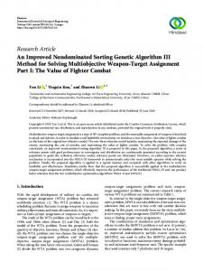
Step 2.4. Choose 𝐹𝑖 to population 𝑃𝑡+1 , until the size of population 𝑃𝑡+1 exceeds 𝑁; the last nondominated set is 𝐹𝑘 . Step 2.5. Crowding distance sorting for every individual in 𝐹𝑘 , choose the best solutions of 𝑁 − |𝑃𝑡+1 | to fill all population slots. Step 2.6. Use the selection, crossover, and mutation operators for 𝑃𝑡+1 to create a new population 𝑄𝑡+1 . Step 3. End, the Pareto front is formed. 3.3. Demand Simulation and UE Solution Algorithm. To handle travel demand uncertainty in the model, stochastic sampling technique is used to simulate uncertain OD demand based on a probability distribution with predefined expectation and variance. In this study, Monte Carlo simulation is used to generate random OD demand according to a truncation normal distribution. The parameters used are the expectation and variance coefficient in the distribution. It should be noted that other distributions could also be used. The potential OD demand is chosen as the only key exogenous input variables to reflect the uncertainty of travel demand. Under every scenario of OD demand realization, the UE model in lower-level is solved using Frank-Wolfe method presented in Sheffi [20]. 3.4. Algorithm Procedure for MDNDP. The algorithm procedure for MDNDP is proposed in Figure 1 and discussed in the following. Step 1 (initialization). Consider the following. Step 1.1. Determine the basic settings of GA, including encoding, population size 𝑃, fitness function, crossover
4.1. Basic Settings. The main results of the MDNDP model are demonstrated on a middle-sized network shown in Figure 2, the network of Nguyen and Dupuis [21], which has been extensively used before by researchers for testing NDP. This network has 13 nodes, 19 existing links, 6 new built links, and 4 OD pairs. A solid line indicates an existing link and can be expanded while a dotted line indicates a link which could be new built. The parameters in the case are given as follows. Expectation of all 4 OD demands is 350, and the variance coefficient in truncation normal distribution of every OD demand is 0.2. Here, for every OD demand 50 random samplings are implemented. In NSGA II the binary encoding is used where 1 means new built or improvement on existing links and 0 otherwise. The length of chromosomes is 25. For example, the chromosome 0000010000000000000111111 means link 6 will be expanded and links from 20 to 25 are chosen to be built. The population size is set as 50. Updating generation ranges to 100, the fitness function is calculated by ranking the objective function of all individuals. The selection operator is binary tournament selection. The crossover operator is single-point crossover with probability 0.8 and the mutation operator is single-point mutation with probability 0.01. The parameters 𝛼 = 0.15 and 𝛽 = 4 in BPR function are used. Other settings are shown in Figure 2 and Table 1, including the link indicator, free flow time, existing capacity, planned capacity, and construction cost of every link. 4.2. Experiment Results. Figure 3 shows the Pareto front of the solutions of MDNDP on Nguyen-Dupuis network. Figures from 4 to 6 are the projection of the Pareto front on the axis of standard deviation of TTT, expectation of TTT, and construction cost. The Pareto front here consisted of 50 Pareto optimal solutions. Each dot in the front indicates a different configuration
Mathematical Problems in Engineering
5
∙ Population size P ∙ Evolution generation Nm ∙ Demand sampling size Snp
∙ Initialization
N=1 N= N+1
Implement the NSGA II
p=1 p= p+1 S=1 S= S+1
OD demand sampling
UE assignment Yes Calculate the objectives in upper-level
Yes
S < Snp
No
p