EMOPSO: A Multi-Objective Particle Swarm Optimizer with Emphasis on Efficiency Gregorio Toscano-Pulido1, Luis Vicente Santana-Quintero2 and Carlos A. Coello Coello2 1
Universidad Aut´ onoma de Nuevo Le´ on, AP 34 - F Cd. Universitaria, San Nicol´ as de los Garza, NL 66450, MEXICO 2 CINVESTAV-IPN (Evolutionary Computation Group) Depto. de Computaci´ on, Av. IPN No 2508 Col. San Pedro Zacatenco, M´exico, D.F., 07360, MEXICO {
[email protected]} {
[email protected],
[email protected]}
⋆⋆
Abstract. This paper presents the Efficient Multi-Objective Particle Swarm Optimizer (EMOPSO), which is an improved version of a multiobjective evolutionary algorithm (MOEA) previously proposed by the authors. Throughout the paper, we provide several details of the design process that led us to EMOPSO. The main issues discussed are: the mechanism to maintain a set of well-distributed nondominated solutions, the turbulence operator that avoids premature convergence, the constraint-handling scheme, and the study of parameters that led us to propose a self-adaptation mechanism. The final algorithm is able to produce reasonably good approximations of the Pareto front of problems with up to 30 decision variables, while performing only 2,000 fitness function evaluations. As far as we know, this is the lowest number of evaluations reported so far for any multi-objective particle swarm optimizer. Our results are compared with respect to the NSGA-II in 12 test functions taken from the specialized literature.
1
Introduction
Particle swarm optimization (PSO) has been found to be a very effective engine for multi-objective optimization, and several multi-objective particle swarm optimizers (MOPSOs) have been proposed in the last few years [1]. Nevertheless, very few researchers have studied the basic mechanisms of a MOPSO, aiming to design a more efficient search engine, which achieves competitive performance at a low number of objective function evaluations (see for example [2, 3]). This paper reports a detailed study of a MOPSO previously proposed by the authors in [4]. Such study led us to propose new mechanisms that produced a new MOPSO that only performs 2,000 fitness function evaluations, while solving test problems ⋆⋆
This author is currently affiliated to CINVESTAV-Tamaulipas Laboratorio de Tecnolog´ıas de la Informaci´ on, Carretera a Monterrey Km. 6, Cd. Victoria, Tamps 87261, MEXICO.
of up to 30 decision variables. To the best of the authors’ knowledge, this is the lowest number of fitness function evaluations ever reported for any MOPSO in the specialized literature. Our results are compared with respect to the NSGA-II [5], which is a multi-objective evolutionary algorithm (MOEA) representative of the state-of-the-art in the area.
2
Towards an Efficient MOPSO
In [4], we proposed the use of clustering techniques to improve the performance of a MOPSO. In order to improve the performance of our original algorithm, we performed several modifications to it. As a first step, we incorporated a mechanism to distribute the nondominated solutions obtained by the algorithm. Next, we used a turbulence operator, in order to avoid premature convergence. After that, and in order to maximize the subswarms performance, we performed an experiment to fix the number of subswarms to be adopted.Then, we incorporated a mechanism to handle constraints. Finally, we performed an empirical study of the influence of the C1 , C2 and W parameters, and we proposed a simple methodology to self-adapt these parameters. Each of these componentes will be briefly described in the following subsections. 2.1
Handling well-distributed solutions
The MOPSO proposed in [4] does not impose a bound on the total number of nondominated solutions that it can store. This makes it difficult for the decision maker to choose one of them and also complicates the definition of a baseline to perform fair comparisons with respect to other MOEAs. Researchers have proposed several mechanisms to reduce the nondominated solutions generated by a MOEA (most of them applicable to external archives): clusters [6], adaptive grids [7], crowding [5] and relaxed forms of Pareto dominance [8]. In our case, we implemented two mechanisms: (1) an adaptive grid and (2) a relaxed form of Pareto dominance (ε-dominance). These two mechanisms are described next: – Adaptive Grid: Proposed by Knowles & Corne [7], the adaptive grid is really a space formed by hypercubes. Such hypercubes have as many components as objective functions has the problem to be solved. Each hypercube can be interpreted as a geographical region that contains an n number of individuals. The adaptive grid allows us to store nondominated solutions and to redistribute them when its maximum capacity is reached. – ǫ-dominance: This is a relaxed form of dominance proposed by Laumanns et al. [8]. The so-called ε-Pareto set is an archiving strategy that maintains a subset of generated solutions. It guarantees convergence and diversity according to well-defined criteria, namely the value of the ε parameter, which defines the resolution of the grid to be adopted for the secondary population. The general idea of this mechanism is to divide objective function space into boxes of size ε. Each box can be interpreted as a geographical region that
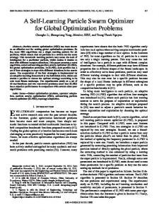
contains a single solution. The approach accepts a new solution into the εPareto set if 1) it is the only solution in the box which it belongs to, 2) it dominates other(s) solution(s) or 3) it competes against other nondominated solution inside the box, but it is closer to the origin vertex of the box. This algorithm is very attractive both from a theoretical and from a practical point of view. However, in order to achieve the best performance, it is necessary to provide the size of the box (the ε parameter) which is problem-dependent, and it’s normally not known before executing a MOEA. Additionally, we also propose a mechanism to distribute nondominated solutions, which is called Hyper-plane distribution. The core idea of this proposal is to perform a good distribution of the hyper-plane space defined by the minima (assuming minimization) from the objectives, and use such distribution to select a representative subset from the whole set of nondominated solutions. The algorithm works as follows: First, it requires as input, a set of nondominated solutions and the quantity n of desirable final solutions. Then, the algorithm selects those solutions which have the minima value on each objective. A hyperplane among all minima solutions is thus computed. Next, the algorithm divides such space into n − 1 regions. Therefore, on the vertex of each region, a perpendicular line to the hyper-plane is computed. Finally, the algorithm only accepts those solutions which are closest to each line. This algorithm has a complexity O(N 2 ), because each individual is compared against everybody else with respect to distance. In Figure 1, we can see an example that aims to clarify the algorithm’s description. In this example, two objective functions are used. Five nondominated solutions need to be selected. So, the hyper-plane (a line in this case) formed by the minima of objective 1 and objective 2 is divided into 4 line segments. Then, each vertex is projected towards the Pareto front. Finally, the solutions closest to those projected points are selected. A First Comparative Study The three approaches previously described to select the best distributed nondominated individuals were implemented and called at each generation. Therefore, on each generation we will have the set of nondominated solutions with a bounded and well-distributed subset. The three algorithms were requested to select 50 nondominated solutions each. The scheme based on the ε-Pareto set needs an extra parameter (ε). This parameter was computed in each test function as follows: the algorithm was executed using a total number of iterations of 200. Then, the ε values were manually fine-tuned to find an average of 40 nondominated solutions in each of the 30 executions. Since the aim of this experiment was to observe if there was an approach which performed best, we adopted the Inverted Generational Distance (IGD) metric [9], as a way to estimate how far is the true Pareto front from the solutions obtained. This measure is defined as: pPn 2 i=1 di (1) GD = n
A
A
7
7 B
6
B
6
C
C
5
5
D
4
Objective 2
Objective 2
E FG
3
H I
D E
4
FG
3
H I J
J
2
2
K
K L
1
L
1 M
M N
N
0
0 0
1
2
3
4
5
6
0
7
1
2
3
4
5
6
7
6
7
Objective 1
Objective 1
A
A
7
7 B
6
6 C
5
5
D
Objective 2
Objective 2
E
4
FG
3
H I
D
4 3
H
J
2
2 K L
1
L
1 M
N
N
0
0 0
1
2
3
4
5
6
7
0
Objective 1
1
2
3
4
5
Objective 1
Fig. 1. Graphical representation of the hyper-plane distribution.
where n is the number of nondominated vectors found by the algorithm being analyzed and di is the Euclidean distance (measured in objective space) between each of these and the nearest member of the true Pareto front. It should be clear that a value of GD = 0 indicates that all the elements generated are in the true Pareto front of the problem. Therefore, any other value will indicate how “far” we are from the global Pareto front of our problem. This metric, also, penalizes when the solutions obtained do not cover completely the true Pareto front. For this first study, we adopted 8 test functions taken from the specialized literature: ZDT1, ZDT2, ZDT3, ZDT4, ZDT6 proposed by Zitzler et al. in [10], Kursawe’s problem proposed in [11], and Deb and Deb2, proposed in [12]. In Table 1, we can see that the adaptive grid was the worst choice, and that the Hyper-plane Distribution outperformed the ε-Dominance approach mainly because of its property of selecting a fixed number of solutions (while we can only estimate the total number of solutions when using ε-dominance). Therefore, we will use the Hyper-plane distribution in our MOPSO. Table 2 shows the average of nondominated solutions found in the last generation by each approach. We can see in this table, that ε-dominance was the algorithm that had more problems to reach the target (40 nondominated solutions). 2.2
Avoiding Premature Convergence
Frans van den Bergh [13] discovered a potentially dangerous property in PSO: if the position of the particles coincides with gbest, then it will move away from the
Approach Function Adaptive-Grid ǫ-Dominance Hyper-plane Distribution ZDT1 0.002855236 0.00149249 0.002029507 ZDT2 0.031790172 0.033058091 0.023006512 ZDT3 0.007237485 0.005816599 0.005786199 2.763645000 2.903810666 2.715304000 ZDT4 ZDT6 0.000224374 0.000186435 0.000197410 Kursawe 0.009648260 0.008716252 0.007975956 0.001454523 0.001606147 0.000475256 Deb Deb2 0.00942435 0.009346694 0.009427080 Table 1. Comparison of results of three approaches to maintain a good distribution of nondominated solutions (adaptive grid, ε-dominance and hyper-plane distribution) with respect to the Inverted Generational Distance metric.
Approach Function Adaptive-Grid ε-Dominance Hyper-plane Distribution ZDT1 39 37 40 ZDT2 24 19 27 ZDT3 38 29 37 ZDT4 2 2 2 40 42 39 ZDT6 Kursawe 40 33 39 Deb 40 36 40 Deb2 39 34 37 Table 2. Comparison of the number of reported solutions at the end of the executions by each of the three approaches.
gbest if the inertia or the current velocity is non-zero. This may lead to premature convergence (i.e. all the particles will converge to the gbest particle, which is usually a local minimum). To determine how often this behavior occurred in our algorithm, we counted how many times a particle’s position was the same than the gbest position in all the executions for all the test functions adopted. In Table 3, we can see the results of this experiment. Frans van den Bergh proposed a new parameter to address this issue, but his proposal is hard to adopt in a multiobjective approach based on Pareto ranking, since we would have to deal with several “best” solutions. Therefore, in [14], we proposed the use of a turbulence operator. This turbulence operator consists of an alteration to the flight velocity of a particle.1 This modification is performed in all the dimensions (i.e., in all the decision variables), such that the particle can move to a completely isolated region. The turbulence operator acts based on a probability factor that considers the current generation and the total number of iterations to be performed. The idea is to have a much higher probability to perturb the flight of the particles at the beginning of the search, and decrease it as we progress in the search. The turbulence can be seen as a mutation operator and it is based on the following expression: temp = current generation/total generations probturbulence = temp1.7 − 2.0 × temp + 1.0
(2) (3)
where temp is used as a temporary variable, current generation is the current generation number, total generations is the total number of generations and probturbulence refers to the probability of affecting the flight of a particle using the turbulence operator. The values used for this expression were empirically derived after a set of experiments. The details of the experiments that led us to this setup may be found in [2]. 2.3
Maximizing the Spread
The appropriate selection of leaders is essential for the good performance of a MOPSO. If the particle chooses an inappropriate leader (i.e., a leader who is too far away in the search space) then most of the flight will be fruitless because the particle will not be visiting promissory regions of the search space. In [4], we proposed to use not one but several swarms to avoid this type of problem (in order to make a difference between the use of the word swarm from traditional PSO’s approaches, and the use of several swarms, from our approach, we introduce the word subswarm, which means a set of particles that has its own PSO’s behavior. The subswarms share information among them by interchanging their leaders with certain probability). However, we did not provide any statistical analysis related to the number of subswarms needed. 1
This mechanism is inspired on the one proposed in [15].
Thus, we proceeded to perform such an analysis. Table 4 summarizes the results obtained, showing the mean of 30 independently executions of the algorithm using 2,000 fitness function evaluations. Each execution was tuned to perform 2, 000 fitness function evaluations. We found that by using 8 subswarms, the algorithm exhibited its best performance in 5 out of 8 test functions. We think, that the use of this value can be beneficial most of the time. Therefore, we adopted it as the default value for the number of subswarms. It is important to note that this experiment was performed using 40 particles, which means that each subswarm will have 5 particles. Because of the results, we suggest to use 8 subswarms as a fixed parameter in our algorithm. Statistics Particle = GBest Mean 104.81192 Best 2 729 Worst St.dev. 110.59983 Median 74 Table 3. Statistical results obtained from the counting of the cases in which the particle was equal to its gbest.
Subswarms (clusters) Function 1 2 4 8 20 ZDT1 0.004820567 0.005645242 0.004388993 0.002853130 0.003191553 ZDT2 0.034759800 0.013606517 0.017762557 0.012582413 0.013187440 ZDT3 0.016337620 0.017927403 0.017630486 0.008787392 0.011176582 ZDT4 4.536191000 3.445736000 3.27696600 3.7399510000 3.762421666 ZDT6 0.003337423 0.000509384 0.000472352 0.000334933 0.000431701 Kursawe 0.069521400 0.04149130 0.043504603 0.0498330600 0.042813556 Deb 0.034178800 0.009745156 0.007927125 0.007114026 0.008663098 Deb2 0.009801385 0.009445994 0.00889158 0.008950303 0.009510023 Table 4. Results of the impact of the number of clusters on each test function, with respect to Inverted Generational Distance metric.
2.4
A Constraint-Handling Mechanism
Since the approach proposed in [4] does not use any special mechanism to deal with constrained search spaces, we incorporated the mechanism proposed in [14]. This approach does not require any user-defined parameters and it performs less objective function evaluations than any of the other approaches with respect to which it was compared, while obtaining similar results (see [14] for further details).
2.5
Analyzing the Impact of the PSO’s Parameters
The PSO algorithm has three parameters that play a key role in the algorithm’s behavior: 1. W: velocity inertia 2. C1: cognitive component 3. C2: social component The fact that a MOEA converges to a set of solutions rather than to a single value, makes it difficult to perform an statistical analysis such as the analysis of variance, which can determine how sensitive is an algorithm to its parameters. Nevertheless, we performed a very thorough analysis of parameters (similar to an analysis of variance), with the aim of finding the best possible parameter configuration for our approach (considering the set of test functions adopted). It is worth indicating that the parameters settings that have been previously proposed (see for example [16]) for the original (unconstrained single-objective) PSO, do not provide a good performance in the context of multiobjective optimization and therefore the motivation to perform the thorough analysis reported in [2]. In order to analyze the impact of the parameters on our proposed approach, we considered several configurations, and performed an exhaustive analysis. The configurations adopted are: W = {0.0, 0.1, 0.2, 0.3, 0.4, 0.5, 0.6, 0.7, 0.8, 0.9, 1.0} C1 = {1.0, 1.2, 1.4, 1.6, 1.8, 2.0, 2.2, 2.4, 2.6, 2.8, 3.0} C2 = {1.0, 1.2, 1.4, 1.6, 1.8, 2.0, 2.2, 2.4, 2.6, 2.8, 3.0}
(4)
For all our experiments, we adopted 40 particles. However, we analyzed three different performance scenarios: 1. Experiment 1: Use of a randomly generated initial population and a low number of fitness function evaluations (we used Gmax = 25, which gives us a total of 1000 fitness function evaluations). 2. Experiment 2: Use of a good approximation of the Pareto front in the initial population. In all the experiments performed in this case, the same approximation was fed to the algorithm in its initial generation. In this case, we only performed 600 fitness function evaluation (Gmax = 15), since we were interested in analyzing the capability (or possible difficulties) of our algorithm to reach the true Pareto front of a problem once a good (and sufficiently close) approximation had been produced. 3. Experiment 3: Use of a large number of fitness function evaluations (Gmax = 250, which gives a total of 10, 000 fitness function evaluations) in order to assess the performance of our approach in the long term. We adopted eleven test functions for Experiment 1 and Experiment 2. Due to the high CPU time required by each run, we only adopted six test functions for Experiment 3. Since we needed to assess performance in each case, we chose the inverted generational distance metric, since it can measure both
closeness to the true Pareto front and spread of solutions. An obvious problem with so many experiments was how to present the results in a compact form. For that sake, we adopted a set of squares (called “mosaics”), such that each of them has a gray scale that corresponds to the mean value of the inverted generational distance over 30 independent runs, produced from one combination of {W,C1,C2} (all the possible combinations were adopted, considering the sets of possible values previously defined for these three parameters). The mean results were normalized between zero and 255 (where zero is the best possible value and 255 is the worst). The results of each of the three above experiments are briefly discussed next, but the mosaics themselves could not be included due to space restrictions; however, they can be found in [2]. Conclusions from the Second Series of Experiments After combining the results from the three experiments, we concluded the following: – The best range for C1 and C2 is from 1.2 to 2.0. From within this range, we can say that C1=C2=1.4 provides the best overall performance. – The best values for W are those less or equal to 0.5. – Note, however, that the above values do not produce the best possible performance in all cases (as expected, because of the No Free Lunch Theorem [17]). This is precisely what motivated us to propose a mechanism to self-adapt the parameters of our approach so that it automatically adjusts the parameters according to the characteristics of the search space being explored. 2.6
Self-Adaptive Mechanism
The results obtained from the experiments reported in the previous subsection led us to propose a self-adaptive mechanism which is described in this subsection. We proposed the use of a traditional proportional selection mechanism to select the most appropriate combination of parameters values to be adopted. We adopted roulette-wheel selection for that sake [18]. Rather than computing fitness for each combination of values, we count the number of nondominated solutions generated by each combination of values. Let’s assume that the parameter W can take 3 possible values: 0, 0.5, 1.0. So, at the beginning of the search, each value has a 33% probability of occurring (see Figure 2 (a)). At generation zero, each possible value has a “fitness” of one. Now, let’s assume that after one generation, W = 0 generates 2 new nondominated solution, W = 0.5 generate 4 new nondominated solution and W = 1 did not contribute with any new nondominated solution. Thus, we reward the “fitness” of W=0.5 by increasing its value in 0.4 (we increase fitness in 0.1 for each new nondominated solution produced). So, W = 0.5 now has a fitness of 1.4. Analogously, W = 0 has a fitness of 1.2 and W = 1 remains with a fitness of 1.0. The new share in the roulette wheel for each value is shown in Figure 2 (b). Since the total fitness is now 3.6 (1.4 + 1.2 + 1.0), the share of each value is: W = 0.5 (1.4/3.6), W = 0 (1.2/3.6) and W = 1 (1.0/3.6). After generation two, W = 0.5 generated one
new nondominated solution, the same happened with W = 1.0 and W = 0 did not produce any new nondominated solutions. So, W = 0.5 now has a fitness of 1.5, W = 1.0 has a fitness of 1.1 and W = 0 remains with a fitness of 1.2. Thus, the total fitness is now 3.8, and we have the following: W = 0.5 has a share of 1.5/3.8, W = 1 has a share of 1.1/3.8 and W = 0 has a share of 1.2/3.8 (see Figure 2 (c)). B)
A) First Generation
Prob: 1/3
Second Generation
Prob: 1.2/3.6
Prob: 1/3
Prob: 1.4/3.6
Value: 0.0 Value: 0.5
Value: 0.0 Value: 0.5 Prob: 1/3
Prob: 1/3.6
Value: 1.0
Value: 1.0 C) Third Generation Prob: Prob: 1.2/3.8 1.5/3.8
Value: 0.0
Value: 0.5
Prob: 1.1/3.8
Value: 1.0
Fig. 2. Roulette wheel selection example at the a) first, b) second and c) third generation.
To validate our proposal, we compare it against two other parameter selection mechanisms: a) deterministic selection and b) random selection. Deterministic selection : C1, C2 and W are deterministically set to 1.4, 1.4 and 0.2, respectively (these values are the center of the region which performed best from the experiments reported in the previous subsection). Random selection : C1, C2 and W pick their values randomly from an interval from 1.2 to 2 for C1 and C2 and from the range from 0.0 to 0.4 for W (this is the range of values which performed best in the experiments reported in the previous subsection). The detailed results from this experiment can be seen in [2]. Although the results of this study seem inconclusive, we argue that the use of a self-adaptive mechanism for adjusting the parameters gives a better performance in a wider range of functions, and avoids that the user has to setup the parameters of the algorithm by hand. In this experiment, most of the time, the approach which
performed best for 25 generations, was also the best performer when adopting 50 and 250 generations. So, we argue, that the proposal to self-adapt the parameters improved the overall performance of the algorithm. After introducing this last component (i.e., the self-adaptive mechanism), the final version of our proposed algorithm, which we call Efficient Multi-Objective Particle Swarm Optimizer (EMOPSO) is shown in flowchart 3. This approach does not require any manual fine-tuning of its PSO parameters.
3
Test Problems
Deb et al. [19] proposed a set of constrained multiobjective problems in which the difficulty can be controlled by varying a set of parameters. In this study, we use g(x) = 1 + x1 for the test problems CTP1 to CTP7, a1 = 0.858, b1 = 0.541, a2 = 0.728, and b2 = 0.295 for CTP1 and the parameters shown in Table 5 for CTP2 to CTP7. Problem CTP2 CTP3 CTP4 CTP5 CTP6 CTP7
θ −0.2π −0.2π −0.2π −0.2π −0.1π −0.05π
a 0.2 0.1 0.75 0.1 40.0 40.0
b 10.0 10.0 10.0 10.0 0.5 0.5
c 1.0 1.0 1.0 2.0 1.0 1.0
d 6.0 0.5 0.5 0.5 2.0 2.0
e constraints boundaries 1.0 2 0 ≤ x1 , x2 ≤ 1 1.0 1 0 ≤ x1 , x2 ≤ 1 1.0 1 0 ≤ x1 , x2 ≤ 1 1.0 1 0 ≤ x1 , x2 ≤ 1 -2.0 1 0 ≤ x1 ≤ 1, 0 ≤ x2 ≤ 10 -2.0 1 0 ≤ x1 ≤ 1, 0 ≤ x2 ≤ 10
Table 5. Parameters chosen for CTP2 to CTP7
4
Comparison of Results
In order to allow a quantitative assessment of results, we adopted the following performance measures: Inverted Generational Distance [9], Two Set Coverage [10] and the Spread metric [5]. We compare results with respect to the NSGA-II using 12 standard test functions: 7 from the Constrained Test Problems (CTP1 to CTP7) proposed by Deb et al. [19], which were previously discussed; and 5 from the ZDTs test problems proposed by Zitzler et al. in [10]. The detailed description of these 12 test functions was omitted due to space restrictions. The CTPs problems all have 2 decision variables each, and the ZDTs functions are unconstrained and have between 10 (ZDT4 and ZDT6) and 30 (ZDT1, ZDT2 and ZDT3) decision variables. ZDT5 is not included in our study because it is a binary function, and we only adopted test functions in which the decision variables are real numbers. In the following examples, the NSGA-II was run using a population size of 40, a crossover rate of 0.9, tournament selection, a mutation rate of 1/N , where N = number of variables (real numbers representation was
adopted), a distribution index of 15 for SBX, and a distribution index of 20 for its parameter-based mutation operator. Our EMOPSO used 40 particles and a total of 8 swarms. The total number of fitness function evaluations was set to 2, 000 for the two algorithms compared (50 generations).
Function CTP1 CTP2 CTP3 CTP4 CTP5 CTP6 CTP7 ZDT1 ZDT2 ZDT3 ZDT4 ZDT6
IGD EMOPSO NSGA-II Mean σ Mean σ 0.0004 0.0001 0.0013 0.0014 0.0014 0.0003 0.0094 0.0056 0.0084 0.0016 0.0100 0.0035 0.0327 0.0163 0.0417 0.0121 0.0060 0.0012 0.0102 0.0064 0.002 0.0006 0.0096 0.0108 0.0002 0.0006 0.0017 0.0027 0.0022 0.0001 0.0740 0.0177 0.0007 0.0003 0.1938 0.0632 0.0020 0.0005 0.061 0.011 8.1128 5.1184 5.5563 1.8295 0.0980 0.1191 0.6098 0.1447
Set Coverage EMOPSO NSGA-II Mean σ Mean σ 0.0868 0.0393 0.2133 0.0657 0.3208 0.0698 0.3266 0.0811 0.5275 0.1788 0.6242 0.1223 0.1465 0.2039 0.7294 0.1814 0.3933 0.1404 0.4808 0.1135 0.1113 0.0643 0.2041 0.0612 0.0042 0.0132 0.0741 0.0480 0 0 1 0 0 0 1 0 0 0 1 0 0.0531 0.2018 0.4438 0.3703 0 0 1 0
Spread EMOPSO NSGA-II Mean σ Mean σ 0.1957 0.0104 0.2859 0.0386 0.3932 0.0682 0.4210 0.0320 0.5959 0.1253 0.6191 0.080 0.7585 0.2583 0.9909 0.1401 0.5126 0.1054 0.4925 0.0770 0.8679 0.0575 0.3067 0.0707 0.7112 0.1874 0.9998 0.0633 0.0870 0.0164 0.5627 0.0756 0.0755 0.0980 0.7585 0.0757 0.5011 0.0290 0.7033 0.0609 0.9978 0.0081 0.9856 0.0128 0.4380 0.2798 0.8799 0.0775
Table 6. Comparison of results between our approach (EMOPSO) and the NSGA-II.
Table 6 shows that the results obtained by our EMOPSO were superior to those generated by the NSGA-II. Our EMOPSO outperformed the NSGA-II in all the test problems with respect to the set coverage metric, and in all but one (ZDT4) with respect to the inverted generational distance metric. Regarding spread, our approach outperformed the NSGA-II in most problems (except for CTP5, CTP6 and ZDT4). Obviously, if allowed to perform a higher number of fitness function evaluations, the NSGA-II would be able to converge to the true Pareto front of most of these test functions, but our main purpose was to show that our EMOPSO is a viable choice when dealing with objective functions whose computational cost is very high (e.g., in aerospace engineering). Due to space restrictions, the Pareto fronts obtained in each case are not included in the paper.
5
Conclusions and Future Work
Our main conclusions are the following: – We found that the use of subswarms promotes local search as an emergent behavior in our EMOPSO. Consequently, the performance of our approach was improved by the use of subswarms, particularly in the presence of disconnected Pareto fronts. – We have proposed a mechanism called “hyper-plane distribution”, to distribute nondominated solutions. – The use of a perturbation mechanism in our multiobjective particle swarm optimizer was found to be critical to control its high selection pressure, as to avoid premature convergence.
– In general, we found that it is quite difficult to find fixed values for the three most significant parameters of our approach (W, C1 and C2). It is worth indicating that the comprehensive study of parameters that we performed is, as far as we know, the first of its type (in the context of multiobjective particle swarm optimization). Based on the results of this study, we designed a self-adaptive mechanism for these parameters, and we found this to be a good alternative to facilitate the use of our approach. Some possible paths to extend this work are the following: – Experiment with other PSO’s models and with different interconnection topologies. – Study alternative methods for the survivor selection mechanism. – Study alternative (perhaps more elaborate) constraint-handling mechanisms. – Study alternative mechanisms to accelerate convergence while keeping the same quality of results achieved by our EMOPSO. – Study alternative mechanisms to distribute nondominated solutions. – To assess the performance of our EMOPSO in a real-world problem in which the cost of evaluating the objective functions is very high (computationally speaking).
Acknowledgments The second author acknowledges support from CONACyT through project number 45683-Y. The third author acknowledges support from CONACyT through a scholarship to pursue graduate studies at the Computer Science Department of CINVESTAV-IPN.
References 1. Reyes-Sierra, M., Coello Coello, C.A.: Multi-Objective Particle Swarm Optimizers: A Survey of the State-of-the-Art. International Journal of Computational Intelligence Research 2(3) (2006) 287–308 2. Toscano Pulido, G.: On the Use of Self-Adaptation and Elitism for Multiobjective Particle Swarm Optimization. PhD thesis, Computer Science Section, Department of Electrical Engineering, CINVESTAV-IPN, Mexico (2005) 3. Branke, J., Mostaghim, S.: About Selecting the Personal Best in Multi-Objective Particle Swarm Optimization. In Runarsson, T.P., Beyer, H.G., Burke, E., MereloGuerv´ os, J.J., Whitley, L.D., Yao, X., eds.: Parallel Problem Solving from Nature - PPSN IX, 9th International Conference. Springer. Lecture Notes in Computer Science Vol. 4193, Reykjavik, Iceland (2006) 523–532 4. Toscano Pulido, G., Coello Coello, C.A.: Using Clustering Techniques to Improve the Performance of a Particle Swarm Optimizer. In et al., K.D., ed.: Genetic and Evolutionary Computation–GECCO 2004. Proceedings of the Genetic and Evolutionary Computation Conference. Part I, Seattle, Washington, USA, SpringerVerlag, Lecture Notes in Computer Science Vol. 3102 (2004) 225–237
5. Deb, K., Pratap, A., Agarwal, S., Meyarivan, T.: A Fast and Elitist Multiobjective Genetic Algorithm: NSGA–II. IEEE Transactions on Evolutionary Computation 6(2) (2002) 182–197 6. Zitzler, E., Thiele, L.: Multiobjective Evolutionary Algorithms: A Comparative Case Study and the Strength Pareto Approach. IEEE Transactions on Evolutionary Computation 3(4) (1999) 257–271 7. Knowles, J.D., Corne, D.W.: Approximating the Nondominated Front Using the Pareto Archived Evolution Strategy. Evolutionary Computation 8(2) (2000) 149– 172 8. Laumanns, M., Thiele, L., Deb, K., Zitzler, E.: Combining Convergence and Diversity in Evolutionary Multi-objective Optimization. Evolutionary Computation 10(3) (2002) 263–282 9. Veldhuizen, D.A.V.: Multiobjective Evolutionary Algorithms: Classifications, Analyses, and New Innovations. PhD thesis, Department of Electrical and Computer Engineering. Graduate School of Engineering. Air Force Institute of Technology, Wright-Patterson AFB, Ohio (1999) 10. Zitzler, E., Deb, K., Thiele, L.: Comparison of Multiobjective Evolutionary Algorithms: Empirical Results. Evolutionary Computation 8(2) (2000) 173–195 11. Kursawe, F.: A Variant of Evolution Strategies for Vector Optimization. In Schwefel, H.P., M¨ anner, R., eds.: Parallel Problem Solving from Nature. 1st Workshop, PPSN I. Volume 496 of Lecture Notes in Computer Science Vol. 496., Berlin, Germany, Springer-Verlag (1991) 193–197 12. Deb, K.: Multi-Objective Genetic Algorithms: Problem Difficulties and Construction of Test Problems. Evolutionary Computation 7(3) (1999) 205–230 13. van den Bergh, F.: An Analysis of Particle Swarm Optimization. PhD thesis, Faculty of Natural and Agricultural Science, University of Petoria, Pretoria, South Africa (2002) 14. Toscano-Pulido, G., Coello Coello, C.A.: A Constraint-Handling Mechanism for Particle Swarm Optimization. In: Proceedings of the Congress on Evolutionary Computation 2004 (CEC’2004). Volume 2., Piscataway, New Jersey, Portland, Oregon, USA, IEEE Service Center (2004) 1396–1403 15. Fieldsend, J.E., Singh, S.: A Multi-Objective Algorithm based upon Particle Swarm Optimisation, an Efficient Data Structure and Turbulence. In: Proceedings of the 2002 U.K. Workshop on Computational Intelligence, Birmingham, UK (2002) 37–44 16. Kennedy, J., Eberhart, R.C.: Swarm Intelligence. Morgan Kaufmann Publishers, San Francisco, California (2001) 17. Wolpert, D.H., Macready, W.G.: No Free Lunch Theorems for Optimization. IEEE Transactions on Evolutionary Computation 1(1) (1997) 67–82 18. Goldberg, D.E.: Genetic Algorithms in Search, Optimization and Machine Learning. Addison-Wesley Publishing Company, Reading, Massachusetts (1989) 19. Deb, K., Pratap, A., Meyarivan, T.: Constrained Test Problems for Multi-objective Evolutionary Optimization. In Zitzler, E., Deb, K., Thiele, L., Coello, C.A.C., Corne, D., eds.: First International Conference on Evolutionary Multi-Criterion Optimization. Springer-Verlag. Lecture Notes in Computer Science No. 1993 (2001) 284–298
Fig. 3. Flowchart of the proposed algorithm.