2009 International Joint Conference on Computational Sciences and Optimization
A Particle Swarm Optimizer with Multi-Stage Linearly-Decreasing Inertia Weight Jianbin Xin 1, 2, Guimin Chen 1, Yubao Hai 1 1 School of Mechatronics, Xidian University, Xi’an 710071, China 2 School of Electrical Engineering, Xi’an Jiaotong University, Xi’an 710049, China
[email protected];
[email protected]
Comprehensive Learning Particle Swarm Optimizer (CLPSO) [8] and the Fully Informed Particle Swarm Optimizer (FIPSO) [9], have shown remarkable performance in consistently finding the global optimum. But their superiority always reveals after 3000 or more iterations. Therefore, the effects of nonlinear strategies on PSOs in relatively long runs should be evaluated. The present work proposes a new group of nonlinear strategies called multi-stage linearly-decreasing inertia weight (MLDW), for the purpose of easily refining the decreasing process of the inertia weight. Six commonly used benchmarks are used to evaluate MLDW for 5000 iterations.
Abstract The inertia weight is often used to control the global exploration and local exploitation abilities of particle swarm optimizers (PSO). In this paper, a group of strategies with multi-stage linearlydecreasing inertia weight (MLDW) is proposed in order to get better balance between the global and local search. Six most commonly used benchmarks are used to evaluate the MLDW strategies on the performance of PSOs. The results suggest that the PSO with W5 strategy is a good choice for solving unimodal problems due to its fast convergence speed, and the CLPSO with W5 strategy is more suitable for solving multimodal problems. Also, W5-CLPSO can be used as a robust algorithm because it is not sensitive to the complexity of problems for solving.
2. Particle Swarm Optimizers 2.1. LDW-PSO
1. Introduction
PSO is a population-based algorithm. Each individual in the population is called a particle. In a ddimension search space, the position vector and the velocity vector of the ith particle can be represented as Xi = (xi1, xi2, ... , xid) and Vi = (vi1, vi2, ... , vid) respectively. The best position found by the ith particle so far is denoted as Pi = (pi1, pi2, ..., pid), and the best position found by the whole swarm as Pg = (pg1, pg2, ... , pgd). The velocity and position of the ith particle in the kth dimension are updated as follows: vik = wvik + c1R1 () * ( pik − xik ) + c2 R2 () * ( pgk − xik ) (1)
The Particle Swarm Optimizer (PSO) is an evolutionary computation technique first introduced by Kennedy and Eberhart in 1995 [1]. Because of its simple mechanism and high performance, PSO has been used in many engineering fields such as neural network training, reactive power compensation [2] and task scheduling [3]. As an important parameter in PSO, the inertia weight is often used to balance global exploration and local exploitation of the searching process. PSO with linearly-decreasing inertia weight (LDW-PSO) [4] was recommended due to its good performance over a large number of optimization problems. Nonlinearlydecreasing strategies of inertia weight also have been proposed and evaluated [5-7]. However, the evaluation of these nonlinear strategies was drawn based on relatively short runs (e.g., 1000 or 2000 iterations) on classic benchmarks. It’s should be noted that some algorithms might outperform others by finding a locally best region of a multimodal function in a short run. Furthermore, recent PSO variants, including the
978-0-7695-3605-7/09 $25.00 © 2009 IEEE DOI 10.1109/CSO.2009.420
xik = xik + vik
(2)
where w is the inertia weight, c1 and c2 are constants known as acceleration coefficients, which are often fixed at 2, and R1() and R2() are two random numbers in the range [0, 1]. In LDW-PSO, w is given as (3) w = ( ws − we )(t max − t ) / t max + we where tmax donates the maximum number of allowable iterations, t represents the current iteration times, and ws and we are the initial and final values of the inertia 505
Authorized licensed use limited to: XIDIAN UNIVERSITY. Downloaded on September 14, 2009 at 23:53 from IEEE Xplore. Restrictions apply.
weight, respectively. The performance of LDW-PSO can be improved significantly when ws=0.9 and we=0.4 [4].
4. Test 4.1. Benchmarks
2.2. CLPSO
Six commonly used benchmarks were adopted to evaluate the performance of algorithms. (1) Sphere function:
In CLPSO [8], the velocity of particle i in the kth dimension is updated as (4) vik = wvik + c3 R3 () * ( p Fi ( k ) k − xik )
d
f1 ( x) =
where Fi(k) defines which particles’ pik should particle i follow in the kth dimension.
∑x
2 i
i =1
(2)Rosenbrock function:
∑ [100( x d
3. MLDW strategies
f 2 ( x) =
i +1
− x i2 ) 2 + ( x i − 1) 2
i =1
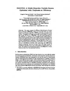
The inertia weight offers PSOs a convenient way to control between exploration and exploitation. In order to find a strategy that can balance the search better between exploration and exploitation over the iterations than LDW does, a group of MLDW is presented, which can be expressed as ⎧(ws − wm )(t1 − t ) / t1 + wm 0 ≤ t ≤ t1 ⎪ w = ⎨wm t1 < t ≤ t2 (5) ⎪(w − w )(t − t ) /(t − t ) + w t < t ≤ t e max max 2 e 2 max ⎩ m where tmax=5000, ws=0.9, we=0.4, and wm, t1 and t2 and the multi-stage parameters The multi-stage parameters of six selected MLDW strategies which are referred to as W1-W6, are listed in Table 1. Figure 1 plots the curves of these strategies.
(3) Rastrigin function: d
f 3 ( x) =
W1 0.8 1000 4000
W2 0.8 2000 3000
W3 0.65 1000 4000
W4 0.65 2000 3000
W5 0.5 1000 4000
f 4 ( x) =
0.8
Inertia W eight
− 10 cos( 2πxi ) + 10]
d d 2 x 1 ∑ xi − ∏ cos( i ) + 1 4000 i = 1 i i =1
(5) Schaffer’s f6 function: f 5 ( x) = 0.5 −
(sin x12 + x 22 ) 2 − 0.5 [1 + 0.001( x12 + x 22 )] 2
(6) Ackley function: ⎛ 1 f 6 ( x ) = − 20 exp ⎜⎜ − 0 .2 d ⎜ ⎝
d
∑x i =1
2 i
⎞ ⎟ − exp ⎛⎜ 1 ⎟⎟ ⎜d ⎝ ⎠
⎞
d
∑ cos (2πx i =1
i
)⎟⎟ + 20 + e ⎠
The parameters for each benchmark are given in Table 2.
W6 0.5 2000 3000
4.2. Experimental setting The population size was set at 30 and the symmetric initialization method was used. Each variant of the PSOs was tested 30 times on each benchmark. The optimization results at the 1000th iteration, the 3000th iteration, and the 5000th iteration were recorded, respectively.
W1 W2 W3 W4 W5 W6
0.75
2 i
(4) Griewank function:
0.9 0.85
∑[x i =1
Table 1. Parameters for selected MLDW strategies wm t1 t2
]
0.7
4.3. Results
0.65 0.6
In order to combine the results from different functions, we standardized the results to the same scale using the method proposed in [9]. Because all the benchmarks are minimization problems, negative standardized values are better than average, while positive ones are worse than average. Table 3 and 4 list the standardized results for Wj-PSO and Wj-CLPSO, respectively.
0.55 0.5 0.45 0.4
0
500
1000
1500 2000
2500 3000 3500 Iterations
4000 4500
5000
Figure 1. The inertia weight curves over iterations In the following sections, LDW-PSO is referred to as W0-PSO while PSO with MLDW as Wj-PSO, and CLPSO with LDW as W0-CLPSO while CLPSO with MLDW as Wj-CLPSO.
506
Authorized licensed use limited to: XIDIAN UNIVERSITY. Downloaded on September 14, 2009 at 23:53 from IEEE Xplore. Restrictions apply.
W5-CLPSO is what we want because not only does it reach the goal in relatively short runs, but also its success rate is high up to 100%.
Table 2. Parameters for the benchmarks
(-100, 100) (-30, 30)
(a)
20
10
10-5 0.01
10
-20
10
W3-PSO W -PSO 5 W0-PSO W -CLPSO 3 W5-CLPSO W -CLPSO
-40
10
0
Best Function Value
15 4
x 10
(d)
4
10
-5
10
W3-PSO W5-PSO W0-PSO W3-CLPSO W5-CLPSO W0-CLPSO
-10
10
0
W -PSO 3 W5-PSO W -PSO 0 W3-CLPSO W -CLPSO 5 W0-CLPSO
2
10
0
10
-2
10
-4
5
10
10
15
0
5
10 FEs
4
x 10
(e)
5
15 4
x 10
(f)
0
10
10
-5
Best Function Value
W1-CLPSO W2-CLPSO W3-CLPSO W4-CLPSO W5-CLPSO W6-CLPSO W0-CLPSO
10 FEs
10
FEs
5000 11.542 0.326 -2.455 -1.955 -2.95 -2.788 -1.721
5
x 10
0
10
0
4
(c)
5
-15
3000 5.377 12.344 -3.586 -3.114 -4.233 -3.982 -2.806
10
15
10
Table 4. Standardized results of Wj-CLPSO 1000 2.627 11.904 -5.668 0.03 -7.443 -4.055 2.606
2
0
10 FEs
5000 3.977 -0.474 -1.859 -0.884 -0.377 -0.736 0.354
0
4
10
10
5
Table 3. Standardized results of Wj-PSO 3000 8.434 9.417 -3.87 -3.697 3.780 -3.536 -2.968
6
10
0
-60
1000 3.521 10.398 -5.637 0.759 -8.366 -3.531 2.856
W3-PSO W -PSO 5 W0-PSO W -CLPSO 3 W5-CLPSO W -CLPSO
8
10
0
10
W1-PSO W2-PSO W3-PSO W4-PSO W5-PSO W6-PSO W0-PSO
(b)
10
10
Best Function Value
2 30
0.01 100 100 0.05 0.05
Best Function Value
Schaffer’s f6 Ackley
Goal
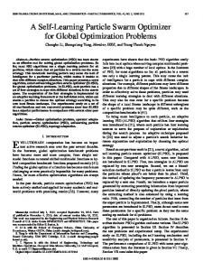
It can be seen from Table 3 and 4 that W3 and W5 (marked in bold) improve PSO and CLPSO either at the 1000th iteration or at the 5000th iteration. Figure 2 shows the mean convergence characteristics of the selected PSO variants, i.e., W0-PSO, W3-PSO, W5PSO, W0-CLPSO, W3-CLPSO and W5-CLPSO. It can be seen from Figure 2 that both W3-PSO and W5-PSO converge faster than W0-PSO at the early stage for all the benchmarks. W3 enhances the searching ability of PSO for Rastrigin and Schaffer f6. Compared with WiCLPSOs, Wi-PSOs can always find good results at the early stage, but are prone to be trapped in a locally optimal region in long runs. For all benchmarks, W3CLPSO and W5-CLPSO surpass other CLPSO variants both in the convergence speed and search accuracy. This indicates that the inertia weight for CLPSO should be decreased quickly at the early stage. The results partially support the conclusion of Chen et al [6] which suggests using concave functions for decreasing strategies. Table 5 presents the iteration times to the goal on average for five of the algorithms mentioned above. The numbers in bold indicate the corresponding success rate is 100%. We may say the performance of
Best Func tion Value
Initialization range (-100, 100) (-30, 30) (-5.12,5.12) (-600, 600) (-600, 600)
Best Function Value
Sphere Rosenbrock Rastrigin Griewank Griewank
Dimensions (d) 30 30 30 10 30
Function
0
10
-5
10
W3-PSO W5-PSO W0-PSO W3-CLPSO W -CLPSO W50-CLPSO
-10
10
0
10
-10
10
W3-PSO W5-PSO W0-PSO W3-CLPSO W -CLPSO W50-CLPSO
-15
10
-20
5
10 FEs
15
10
0
5
(g)
5
10 FEs
4
x 10
15 4
x 10
10
Best Function Value
0
10
-5
10
W3-PSO W5-PSO W0-PSO W3-CLPSO W5-CLPSO W0-CLPSO
-10
10
-15
10
0
5
10 FEs
15 4
x 10
Figure 2.The mean convergence characteristics of six selected PSO variants on the benchmarks. (a) Sphere function. (b) Rosenbrock’s function. (c) Rastrigin’s function. (d) Griewank’s function (10d). (e) Griewank’s function (30d). (f) Schaffer’s f6 function. (g) Ackley’s function. Generally speaking, W5-PSO is suitable for solving unimodal problems such as the Sphere function
507
Authorized licensed use limited to: XIDIAN UNIVERSITY. Downloaded on September 14, 2009 at 23:53 from IEEE Xplore. Restrictions apply.
because of its fast convergence speed, whereas W5CLPSO can be used to solve multimodal problems.
[6] G M Chen, Q Han, J Y Jia. Study on the Strategy of Decreasing Inertia Weight in Particle Swarm Optimization Algorithm (in Chinese). Journal of Xi'an Jiaotong University, 2006, 40 (1): 53-56. [7] A Chatterjee and P Siarry. Nonlinear inertia weight variation for dynamic adaptation in particle swarm optimization. Computers & Operations Research, 2006, 33 (3): 859-871. [8] J J Liang, A K Qin, P N Suganthan, and S Baskar. Comprehensive Learning Particle Swarm Optimizer for Global Optimization of Multimodal Functions. IEEE Transactions on Evolutionary Computation, 2006, 10(3): 281-295. [9] R Mendes, J Kennedy, and J Neves. The fully informed particle swarm: Simpler, maybe better. IEEE Transactions on Evolutionary Computation, 2004, 8(3): 204-210.
Table 5.The iteration times to the goal on average f1 ( x)
W3PSO 2187
W5PSO 1115
W0PSO 3082
W5CLPSO 1489
W0CLPSO 2520
f 2 ( x)
2658
1364
3601
1833
3145
f3 ( x)
1173
791
2607
577
1228
f 4 ( x) (10d)
4004
3991
4670
915
2554
f 4 ( x) (30d) f 5 ( x)
2377 822
1377 546
3421 1501
1494 918
2538 1835
f 6 ( x)
2535
1363
3215
1738
2688
5. Conclusion Motivated by the idea of LDW, the strategy of MLDW is proposed in this paper. The PSO with W5 strategy is a good choice for solving unimodal problems due to its fast convergence speed. The CLPSO with W5 strategy features relatively fast convergence speed and high search accuracy and is suitable for solving multimodal problems. Also, W5CLPSO can be used as a robust algorithm because it is not sensitive to the complexity of problems for solving.
Acknowledgments The authors gratefully acknowledge the financial support from the National Natural Science Foundation of China under Grant No. 50805110 and the China Postdoctoral Science Foundation under Grant No. 20070421110. The authors also want to thank Professor P. N. Suganthan for the code he provided.
References [1] J Kennedy, R Eberhart. Particle swarm optimization. International Conference on Neural Networks. Perth, Australia: IEEE, 1995, 1942-1948. [2] R Eberhart, Y Shi. Particle swarm optimization: developments, applications and resources. Proceedings of the IEEE Congress on Evolutionary Computation. Piscataway, USA: IEEE, 2001, 81-86. [3] A Salman, I Ahmad, S Al-Madani. Particle swarm optimization for task assignment problem. Microprocessors and Microsystems, 2002, 26 (8): 363-371. [4] Y Shi, R Eberhart. Empirical study of particle swarm optimization. International Conference on Evolutionary. Computation. Washington, USA, 1999: 1945-1950. [5] X Zhang, Y Du, G Qin. Adaptive Particle Swarm Algorithm with Dynamically Changing Inertia Weight (in Chinese) Journal of Xi'an Jiaotong University, 2005, 39 (19): 1039-1042.
508
Authorized licensed use limited to: XIDIAN UNIVERSITY. Downloaded on September 14, 2009 at 23:53 from IEEE Xplore. Restrictions apply.