algorithm. 2.2 The Slicing Process. After the point set has been transformed according to step 1, the set is adaptively sliced into thin slabs using the following.
A Multi-Resolution Interactive Previewer for Volumetric Data on Arbitrary Meshes Oliver Kreylos∗
Kwan-Liu Ma∗
Abstract In this paper we describe a rendering method suitable for interactive previewing of large-scale arbitary-mesh volume data sets. A data set to be visualized is represented by a “point cloud,” i. e., a set of points and associated data values without known connectivity between the points. The method uses a multi-resolution approach to achieve interactive rendering rates of several frames per second for arbitrarily large data sets. Lower-resolution approximations of an original data set are created by iteratively applying a pointdecimation operation to higher-resolution levels. The goal of this method is to provide the user with an interactive navigation and exploration tool to determine good viewpoints and transfer functions to pass on to a high-quality volume renderer that uses a standard algorithm.
1
Introduction
Current visualization methods for arbitrary-mesh, volumetric data sets do not allow interactive rendering, or even lowquality previewing, of large-scale data sets containing several million grid points. In most cases, a scientist creates or measures such a data set without a-priori knowledge of where to find the features she is looking for; sometimes, even without knowing what those features are. Volume visualization has proven to be a very helpful tool in these situations. But without interactive navigation and exploration tools, finding features in a very large data set and highlighting them using customized transfer functions is very difficult and timeconsuming. If images of a data set could somehow be rendered at interactive rates, even at relatively poor quality, the navigation process could be sped up considerably.
1.1
Related Work
There are several basic rendering methods for arbitrarymesh volumetric data sets that are geared towards generating high-quality images at the expense of rendering time. These methods include the ray casting algorithm described by Garrity [2], the cell projection algorithm discussed by Lichan and Kaufman [5], the plane-sweep modification of the ray casting algorithm invented by Silva et al. [7], the adaptation of the splatting algorithm for non-rectilinear volumes developed by Mao [3], the polygonal approximation to ray casting presented by Shirley and Tuchman [4], and the slicing approach described by Yagel et al. [6]. Researchers have tried optimizing these algorithms following different approaches. Probably the easiest optimization is subsampling in image space, by generating small images ∗ Center for Image Processing and Integrated Computing (CIPIC), Department of Computer Science, University of California, Davis, One Shields Avenue, Davis, CA 95616–8562, {kreylos,ma,hamann}@cs.ucdavis.edu
Bernd Hamann∗
and duplicating pixels using some reconstruction filter. A more sophisticated approach is utilizing graphics hardware for volume rendering. This has been a major success for rectilinear data sets, where 3D texture mapping can be used to generate images at interactive rates [8]. Yagel et al. [6] developed a similar method that generates slices of tetrahedral mesh data sets and uses hardware-assisted polygon rendering to generate images of and composite these slices. There has also been a considerable amount of work on utilizing massively parallel supercomputers to speed up volume rendering [1, 9, 11].
1.2
Interactive Previewing of Large-Scale Volume Data Sets
We describe a new rendering method for irregular volume data sets that uses multiresolution approximations to trade off image quality against rendering speed. This method does not use the topology information contained in irregular data sets, but attempts to reconstruct images of a data set by looking at the data values at grid vertices only. Obviously, this method only generates approximations, but experiments show that the quality of the generated images, combined with the fact that these images are generated rapidly, is more than sufficient to allow the user to detect and highlight features in a data set quickly, see section 5. After good viewpoints and transfer functions have been determined in the previewing phase, those are passed on to either a highaccuracy rendering method [10] or a high-performance rendering method [11].
1.3
Throwing Away the Topology
To allow rapid rendering of approximations of an arbitrarymesh data set, our algorithm does not take the topology of a given grid into account. Instead, it treats the data set as a cloud of points (with associated data values) without known connectivity. Of course, doing so radically decreases the image quality: without knowledge of the vertex connectivity, any rendering can only be an approximation of the correct image. On the other hand, rendering a point cloud has the following benefits: 1. Since it is only an approximation to begin with, one can select a convenient approximation method that utilizes graphics hardware. 2. The algorithm described in section 2 can easily be parallelized for shared-memory, multi-processor graphics workstations. 3. It is comparatively easy to decimate a point cloud to generate a hierarchy of approximations at multiple levels of resolution. Using these optimizations, and selecting the appropriate hierarchy level for the user’s demands, allows to create an
algorithm that renders approximations of arbitrarily large data sets at interactive frame rates.
2
Point-Based Volume Rendering
The major problem of point-based volume rendering is to generate a continuous image. Rendering all points in the set independently, e.g. using a splatting method, usually does not work. In many irregular data sets, the distances between neighbouring points vary over several orders of magnitude; drawing the point cloud with a fixed-size splatting kernel would induce holes in the image in sparse regions and overpainting in dense regions of the data set. Using variable-shape splatting kernels could solve the problem, but finding out the correct shape to use for a given point is a major task in itself when the connectivity of the points is unknown.
2.1
Rendering a Point Cloud
Our algorithm follows the following basic idea to “fill in” pixel values between neighbouring points: 1. A given point set is transformed such that the viewing direction is along the negative z-axis. This step, called “transformation,” is an additional step to optimize later stages of the algorithm.
2. If a given slab contains less than a pre-defined number of points, or if the slab is “thinner” than a pre-defined thickness δz, the slab is not subdivided any further but passed on to the meshing step. (Actually, the parameter δz is implicitly defined by a maximum subdivision depth.) 3. Otherwise, the slab is sliced into two slabs of half its original thickness. The points inside the original slab are distributed among the two new slabs, and both new slabs are sliced again recursively. In our implementation, the point set is stored in an array of fixed size; each slab is associated with a subarray of points. When slicing a slab, all points in that subarray are re-arranged using a quicksort median step. This possibly involves swapping many points during slicing, but it results in the subdivided slab being represented by two consecutive subarrays of points. This increases locality of reference in later slicing steps and in the meshing and rendering stages. Experiments have shown that the reduction in runtime due to higher cache coherency outweighs the cost of swapping the points. 1)
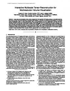
2. The point set is subdivided into thin “slabs” that are orthogonal to the viewing direction, i. e., each slab is of nearly constant z value. We refer to this step as “slicing.” Slicing is done adaptively to take the varying point density in a data set into account. 3. The slabs are converted into a continuous representation (a triangle mesh) by creating the Delaunay triangulation of all points included in the slab. We call this step “meshing.” 4. The meshes associated with each slab are rendered and composited in back-to-front order using hardwareaccelerated polygon rendering and alpha blending. This step is appropriately called “rendering.” These four steps describe a four-stage rendering pipeline, shown in Figure 1. Transformation Point Cloud
Slicing
Transformed Point Cloud
Meshing Slabs
Rendering
Triangulations
Image
Figure 1: The four-stage rendering pipeline defined by our algorithm.
2.2
The Slicing Process
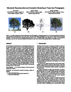
After the point set has been transformed according to step 1, the set is adaptively sliced into thin slabs using the following strategy, see Figure 2: 1. The initial slab contains all points and extends from the minimal to the maximal z value of the point set’s bounding box.
2)
1/1
3)
1/2
1/2
1/2
1/8 1/8
1/4
Figure 2: Adaptively slicing a point set into thin slabs. 1) The initial slab; 2) after one subdivision; 3) final state after three subdivisions. In all three images, the viewing direction is left-to-right. The numbers below each image represent the relative thicknesses of the respective slabs.
2.3
The Meshing Process
After a thin-enough slab has been constructed by the slicing step, it is passed on to the meshing step. This step creates a continuous representation of the points contained in the slab by calculating their Delaunay triangulation. We decided to let the algorithm treat each slab as a single planar triangulation, located halfway between the slab’s minimal and maximal z values. To achieve this, all points inside the slab are projected onto the triangulation’s plane. In our implementation, all points are orthogonally projected in direction of the z axis, and the values associated with the points are not changed in the process. The reason for keeping the point values unchanged is the fact that a triangulation is not meant to be an approximation of a cutting plane through the volume, but it is an approximation of the finite-thickness slab itself. If the former was our goal, the influences of points on the triangulation should be weighed by their distances from it; for our purposes, a slab is more accurately represented when using the original point values. One could imagine the points inside a slab being embedded in clear plastic; viewing the slab from different directions does change the points’ relative positions, but not their values.
Since the planes of all triangulations are orthogonal to the viewing direction, the projections of the points onto the screen are not influenced by this additional projection step when using a parallel viewing projection, and they are only slightly distorted when using a perspective viewing projection, see Figure 3.
Viewing direction
2.4
After the meshing process has created a Delaunay triangulation of the points in a slice, this triangulation is rendered. To render a single triangle, we convert the data values associated with its vertices to color and opacity pairs using a user-defined transfer function, and then draw the triangle into the frame buffer using Goraud shading and α-blending, as provided by standard graphics libraries like OpenGL. Since the slicing process is designed to generate slabs in back-to-front order, and all request queues are ordered by the items’ z-coordinates, the triangulations will be created and rendered in back-to-front order as well. Therefore, using the OpenGL BLEND operator will create an approximation of a ray casting rendering of the data set.
2.5
Slab Figure 3: Projecting all the points inside a slab to the center plane of the slab. Because the projection direction is parallel to the viewing direction, image distortion is minimal. By projecting all points in a slab, the depth ordering of points is destroyed. To generate a high-quality image of a slab, one would have to take this into account and somehow evaluate and save the opacity and color contributions of the cells being “flattened out” by the projection. Our goal, however, is to preview the volume data; experiments have shown that ignoring the influences of projecting the points onto the final image yields sufficient image quality for our purposes. After the projection, our algorithm calculates a Delaunay triangulation of all (projected) points in a slab. To render more consistent images, we want all triangulations to extend to the point set’s bounding box. Our algorithm achieves this by calculating the intersection polygon between a triangulation’s plane and the point set’s bounding box, and inserting the vertices of that intersection polygon into the triangulation as well, see Figure 4.
1)
The Rendering Process
Visible Artifacts
The major cause of visible artifacts in resulting images is the fact that each of the slabs generated by the slicing process is triangulated and rendered independently. This can lead to the effect that the image of one triangulation is not influenced by a point that is very close to the triangulation in object space, but happens to be inside a different slab, see Figure 5. Since the two slabs depicted in Figure 5 are rendered independently, the color and opacity values are interpolated linearly between points P1 and P2 . In a correct rendering, the values would have to be interpolated between points P1 and P3 , and then between points P3 and P2 . But, because point P3 is located in a different slab, the algorithm is oblivious to this fact.
Slab 1 P3 P2
P1
Slab 2 Linear Interpolation
2) Viewing Direction
Figure 5: Potential artifacts in resulting images. Inside slab 2, color and opacity values are wrongly interpolated between points P1 and P2 .
Figure 4: Creating the Delaunay triangulation of a slab. 1) The points inside a slab and the intersection of the triangulation’s plane and the point set’s bounding box (bold); 2) the resulting Delaunay triangulation. The algorithm we use to create a Delaunay triangulation is the randomized incremental algorithm described by Guibas et al. [12].
These artifacts are especially visible when a slab contains only a small number of points, or when all points are clustered in a small region of the triangulation’s intersection with the bounding box of the point set. In these cases, the meshing process connects the points to the vertices on the triangulation’s boundary, and the resulting long and thin triangles will “smear out” the color values all the way to the boundary. The distinct appearance of these visual artifacts is, in some sense, beneficial: it is hard to misinterpret them as features in a data set. Since detecting and emphasizing features present in a data set is the major goal of our algorithm,
it is usable in spite of these distortions. The images produced are not intended to be used “as is,” but they provide help in navigating through a large data set, and in finding interesting viewpoints and transfer functions to pass on for subsequent high-quality renderering.
a “front” and a “back” portion, those can be processed in parallel. In the meshing process, all slices are independent of each other and can be created in parallel.
3
As to be expected, the parallel version of our algorithm is considerably faster than the serial version when executed on a shared-memory multi-processor graphics workstation. We have compared the runtimes on a four-processor SGI Onyx2 workstation, and the parallel algorithm cuts down rendering time by a factor of about four, yielding a parallel efficiency of about 90%. It is more surprising that even on a single-processor workstation the parallel version is faster than the serial one. We believe that the multi-threaded version overlaps the processes of mesh creation and mesh rendering. The latter is done completely in hardware, and in the serial version the CPU has to wait for the graphics subsystem to finish rendering, whereas the parallel version can continue to work in the slicing or meshing pipeline stages.
Parallel Rendering
The serial implementation of our algorithm, as described in section 2, is already capable of rendering small data sets (consisting of several thousand points) on a standard graphics workstation, e. g., an SGI O2, at interactive rates of several frames per second, see section 5. To improve the efficiency of the algorithm, we decided to parallelize it for use on multi-processor shared-memory graphics workstations, like SGI Onyx2 workstations. To distribute the workload among the processors, we exploit both functional parallelism inside the rendering pipeline and object-space parallelism.
3.1
Functional Parallelism
To exploit functional parallelism, we decouple the rendering pipeline as shown in Figure 1 by creating separate threads for each stage and connecting the stages by request queues. The first pipeline stage is handled by a single thread, because it requires only a very short amount of time, and parallelizing it would incur too much overhead. The second and third pipeline stages are represented by a pool of worker threads. The final pipeline stage is also done by a single thread, because the triangulated slices have to be rendered in order, and the OpenGL implementation available to us does not support concurrent rendering into a single frame buffer. The overall structure of our parallel pipeline is shown in Figure 6.
Transformation Point Cloud Slicing Request Queue
Slicing
Meshing
Slicing
Meshing
Slicing
Meshing Meshing Request Queue
4
Rendering Image Rendering Request Queue
One detail of our parellel rendering pipeline is not shown in Figure 6: in order to parallelize the inherently recursive slicing process, a slicer thread can also place a slicing request to the slice request queue. If a slicer thread determines that a slab is thin enough or contains few enough points to render, it will put an entry into the meshing request queue. If, on the other hand, the slab has to be subdivided further, it splits the slab and places two new slicing requests, one for each of the two generated slabs, to the slicing request queue. By following this strategy, we achieve good load balancing between the slicing threads.
Object-Space Parallelism
The threads in the slicing and meshing pipeline stages operate independently of each other. Therefore, we achieve object-space parallelism: as soon as a slab is subdivided into
Comparison with the Serial Algorithm
Multiresolution Rendering
Even after having parallelized the volume renderer, it is still not fast enough to render very large data sets containing millions of points. The reason for this is that the methods used in parallelization do not scale well beyond small numbers of processors in a shared-memory system. To achieve our goal of interactive rendering of very large data sets, we have to create smaller approximations to those data sets first and render them instead. When creating a multiresolution approximation hierarchy, the program (or the user) can always specify an appropriate resolution level to trade off image quality against rendering time.
4.1
Figure 6: The parallel rendering pipeline defined by our algorithm.
3.2
3.3
Creating a Hierarchy of Approximations
To create a hierarchy of approximations, we start with the point set of the original data set (and call it level 0) and perform a point decimation algorithm. We call the result level 1 and repeat the decimation algorithm for level i to generate level (i + 1), and so forth. This process terminates when the result of the decimation algorithm is a sufficiently small data set. With current computer performance and interactive rendering in mind, “small” means that the coarsest-resolution level should contain only a few thousand points.
4.2
The Decimation Algorithm
Finding a sufficiently good representation of a given point set using only a fraction of the original points is difficult, especially when the original points are not aligned on a regular grid. In that case, the algorithm could just sub-sample the grid (by only choosing every other point) and would generate a meaningful approximation (modulo aliasing). In the case of arbitrary-mesh data sets, points are not “aligned” and generally do not form a lattice that could be sub-sampled easily. Even worse, point density might vary over several orders of magnitude in a single data set. Therefore, we need an algorithm that resembles the subsampling approach for regular grids, in the sense that it keeps the relative point densities of an approximation similar to the relative point densities of the original data set.
The algorithm we chose to preserve point densities is based on maximum independent sets. To create an approximation, we first calculate a Delaunay tetrahedrization of the original data set. This results in a tetrahedral mesh where each point is connected to all its nearest neighbours by an edge. As a second step we invoke a “mark-and-sweep” algorithm that extracts the maximum set of points such that no two points in the set are direct neighbours of each other in the original data set, see Figure 7. 1)
us to store hierarchies in a space-efficient way that supports progressive transmission. We store approximation hierarchies by storing the points in the coarsest-resolution level Pn first, followed by storing the points in Pn−1 \ Pn , and finally by storing the points in P0 \ P1 , see Figure 8. The space requirements for storing the points in this way are minimal, because every point is written exactly once, and no additional information is stored. Transmission order
2)
P3
P2 \ P 3
P1 \ P 2
P0 \ P 1
Figure 8: Storing a four-level approximation hierarchy in a file. The coarsest-resolution level P3 is stored first.
3)
4)
Furthermore, when such a hierarchy file is transmitted over a thin-band medium, the receiving end can start rendering the coarsest-resolution approximation as soon as the first |Pn | points defining this resolution level have arrived, and it can increase the resolution of the rendering whenever another hierarchy level is completely received in the transmission process.
5
Examples and Results
We have applied our algorithm to several data sets of different sizes and recorded the runtimes for each data set. The original images generated by our algorithm can also be found under the URL http://graphics.cs.ucdavis.edu/~okreylos/Research/ VolumeRendering/index.html. Figure 7: Creating a lower-resolution approximation of a point set by extracting the maximum independent set. 1) The original point set; 2) the original set’s Delaunay triangulation; 3) the point set’s maximum independent set (included points are circled); 4) the decimated point set. The mark-and-sweep algorithm works as follows: we assume that all points in the original set are coloured either black, grey, or white. Initially, all points are black. The algorithm performs the following steps: 1. Place any point from the set into a queue Q. 2. As long as there are points in Q, perform the following steps: (a) Grab the first point p from Q. (b) If p is black, add it to the result set and colour all its direct neighbours white. (c) If p is not grey, add all its direct neighbours to the queue Q. (d) Colour p grey.
4.3
Storage and Progressive Transmission of Approximation Hierarchies
The approximation hierarchies created by the iterated point decimation algorithm form a chain of subsets Pi of an original point set P0 , i. e., Pn ⊂ · · · ⊂ P1 ⊂ P0 . This fact allows
5.1
A Small Data Set
The smallest data set we have used is the result of the simulation of airflow around a wing. It is defined on a tetrahedral grid, consisting of 2,800 vertices and 13,576 tetrahedra. This data set, called “Mavriplis,” was provided by Dimitri Mavriplis and is courtesy of ICASE.
5.2
A Medium-Sized Data Set
A medium-sized data set we have used is the result of an aerodynamic flow simulation as well. It is defined on a tetrahedral grid consisting of 103,064 vertices and 567,862 tetrahedra. This data set, called “Parikh,” was provided by Paresh Parikh and is courtesy of ViGYAN, Inc. Images of this data set from two different viewpoints, rendered at four different resolutions each, are shown in Figures 11 to 14 and 15 to 18. These images demonstrate that even though our algorithm is merely an approximation of volume rendering, the resulting images often capture the most relevant information in the data. As the progressions from Figures 11 to 14 and from Figures 15 to 18 show, reducing the number of points in an approximation decreases image quality considerable, and makes the coarsest-resolution approximations shown here almost useless. The associated decrease in rendering time, on the other hand, allows the user to choose a low-resolution approximation for navigating between viewpoints, and to choose a high-resolution approximation to “zoom in” on the features.
5.3
A Large-Scale Data Set
The largest data set we used so far is the result of a cosmological simulation. It is defined on a hierarchy of rectilinear grids (generated by an adaptive mesh refinement method), consisting of 2,531,452 vertices altogether. This data set, referred to as “Shalf,” was provided by Greg Bryan, Mike Norman and John Shalf from the Laboratory for Computational Astrophysics at NCSA and from Lawrence Berkeley National Laboratory. Images of this data set, rendered at four different resolutions, are shown in Figures 19 to 22.
5.4
Measurements
Table 1 lists the rendering times for the parallel implementation of our algorithm, executed on an SGI Onyx2 workstation having four MIPS R10K processors running at 195 MHz and 512 MB of main memory. The rendered data sets are the ones described in the previous sections. Dataset Mavriplis Parikh
Shalf
# of points 438 2,800 378 2,425 15,804 103,064 6,607 46,261 346,087 2,531,452
time (sec.) 0.01 0.02 0.01 0.02 0.12 0.99 0.05 0.31 2.66 27.35
Table 1: Rendering times for various data sets.
6
Conclusion
To evaluate our point-based rendering method for arbitrarymesh volumetric data sets, we have implemented an experimental application that allows navigating such data sets and creating colour and opacity maps to pass on to other volume rendering programs, see Figures 9 and 10. Our multiresolution approximation technique allows rendering approximations of data sets of varying sizes at interactive frame rates on a four-processor SGI Onyx2 graphics workstation. In our experiments, we found that the rapid rendering achieved by our approach and implementation is a valuable help in finding and highlighting interesting features in an unknown data set quickly. The artifacts described in section 2.5 are visible, especially when rendering low-resolution approximations, but do not hinder the navigation process. As long as final images are generated by a standard highquality volume rendering algorithm, the image distortions induced by our method are of little concern.
7
Acknowledgements
This work was supported by the National Science Foundation under contracts ACI 9624034 and ACI 9983641 (CAREER Awards), through the Large Scientific and Software Data Set Visualization (LSSDSV) program under contract ACI 9982251. We thank the members of the Visualization Group at the Center for Image Processing and Integrated Computing (CIPIC) at the University of California, Davis.
Figure 9: The previewing application: the main view window. The wireframe cube visible in the background can be used to clip uninteresting parts of the data set. We thank Dimitri Mavriplis at ICASE, Paresh Parikh at ViGYAN, Inc. and Greg Bryan, Mike Norman and John Shalf at the Laboratory for Computational Astrophysics at NCSA and Lawrence Berkeley National Laboratory for providing the data sets used as examples. We thank Gunther Weber at CIPIC for help with the AMR file format.
References [1] Challinger, J., Scalable Parallel Volume Ray-Casting for Nonrectilinear Computational Grids, in Proc. 1993 Parallel Rendering Symposium (1993), ACM Press, pp. 81– 88 [2] Garrity, M. P., Raytracing Irregular Volume Data, in Proc. 1990 Workshop on Volume Visualization, special issue of Computer Graphics, vol. 24(5) (1990), pp. 35– 40 [3] Mao, X., Splatting of Non-Rectilinear Volumes Through Stochastic Resampling, in IEEE Transactions on Visualization and Computer Graphics, vol. 2(2) (1996), pp. 156–170 [4] Shirley, P. and Tuchman, A., A Polygon Approximation to Direct Scalar Volume Rendering, in Proc. 1990 Workshop on Volume Visualization, special issue of Computer Graphics, vol. 24(5) (1990), pp. 63–70 [5] Lichan, H. and Kaufman, A. E., Fast Projection-Based Ray-Casting Algorithm for Rendering Curvilinear Volumes, in IEEE Transactions on Visualization and Computer Graphics, vol. 5(4) (1999), pp. 322-332 [6] Yagel, R., Reed, D. M., Law, A., Shih, P. and Shareef, N., Hardware Assisted Volume Rendering of Unstructured Grids by Incremental Slicing, Proc. 1996 Volume Visualization Symposium, ACM SIGGRAPH (1996), pp. 55-62 [7] Silva, C. T., Mitchell, J. S. B. and Kaufman, A. E., Fast Rendering of Irregular Volume Data, in Proc. 1996 Volume Visualization Symposium, ACM SIGGRAPH (1996), pp. 15–22
Figure 10: The previewing application: the transfer function editor window. The top part of the window allows drawing colour and opacity maps. The lower-left part is used to select various drawing tools. The lower-right part supports the selection of start and end colours for direct colour drawing or colour gradients.
[8] Meissner, M., Hoffmann, U. and Strasser, W., Volume Rendering Using OpenGL and Extensions, in Proc. Visualization ’99, pp. 207–526 [9] Williams, P. L., Parallel Volume Rendering Finite Element Data, Proc. Computer Graphics International ’93, Lausanne, Switzerland, June 1993 [10] Williams, P. L., Max, N. L. and Stein, C. M., A High Accuracy Volume Renderer for Unstructured Data, in IEEE Transactions on Visualization and Computer Graphics, vol. 4(1) (1998), pp. 37–54 [11] Ma, K.-L. and Crockett, T. W., A Scalable Parallel Cell-Projection Volume Rendering Algorithm for ThreeDimensional Unstructured Data, in Proc. IEEE Symposium on Parallel Rendering, IEEE Computer Society Press (1997),pp. 95–104 [12] Guibas, L. J., Knuth, D. E., and Sharir, M. Randomized Incremental Construction of Delaunay and Vorono¨ı Diagrams, in Proc. 17th Int. Colloq.—Automata, Languages and Programming, vol. 443 of Springer Verlag LNCS (1990), Springer Verlag, Berlin, pp. 414–431
Figure 11: Visualization of the “Parikh” data set using 103,064 points, rendered in 0.99 seconds.
Figure 14: Visualization of the “Parikh” data set using 378 points, rendered in 0.01 seconds.
Figure 12: Visualization of the “Parikh” data set using 15,804 points, rendered in 0.12 seconds.
Figure 15: Visualization of the “Parikh” data set using 103,064 points, rendered in 0.99 seconds.
Figure 13: Visualization of the “Parikh” data set using 2,425 points, rendered in 0.02 seconds.
Figure 16: Visualization of the “Parikh” data set using 15,804 points, rendered in 0.12 seconds.
Figure 17: Visualization of the “Parikh” data set using 2,425 points, rendered in 0.02 seconds.
Figure 20: Visualization of the “Shalf” data set using 346,087 points, rendered in 2.66 seconds.
Figure 18: Visualization of the “Parikh” data set using 378 points, rendered in 0.01 seconds.
Figure 21: Visualization of the “Shalf” data set using 46,261 points, rendered in 0.31 seconds.
Figure 19: Visualization of the “Shalf” data set using 2,531,452 points, rendered in 27.35 seconds.
Figure 22: Visualization of the “Shalf” data set using 6,607 points, rendered in 0.05 seconds.