Oct 27, 2016 - (e.g. the engine torque or the steering wheel posi- tion). X and U are ..... the preference according to his wishes and on the other hand, Ï can be ...
A Multiobjective MPC Approach for Autonomously Driven Electric Vehicles Sebastian Peitz* , Kai Sch¨afer* , Sina Ober-Bl¨obaum** , Julian Eckstein*** , Ulrich K¨ohler*** , and Michael Dellnitz*
arXiv:1610.08777v1 [math.OC] 27 Oct 2016
*
Department of Mathematics, Paderborn University, Warburger Str. 100, 33098 Paderborn, Germany ** Department of Engineering Science, University of Oxford, Parks Road, Oxford OXI 3PJ, UK *** Hella KGaA Hueck & Co., Beckumer Str. 130, 59552 Lippstadt, Germany
Abstract We present a new algorithm for model predictive control of non-linear systems with respect to multiple, conflicting objectives. The idea is to provide a possibility to change the objective in real-time, e.g. as a reaction to changes in the environment or the system state itself. The algorithm utilises elements from various well-established concepts, namely multiobjective optimal control, economic as well as explicit model predictive control and motion planning with motion primitives. In order to realise real-time applicability, we split the computation into an online and an offline phase and we utilise symmetries in the open-loop optimal control problem to reduce the number of multiobjective optimal control problems that need to be solved in the offline phase. The results are illustrated using the example of an electric vehicle where the longitudinal dynamics are controlled with respect to the concurrent objectives arrival time and energy consumption.
1
paratively low ranges are both gaining increased attention, requiring advanced control algorithms. Control theory has been influenced significantly by the advances in computational power during the last decades. For a large variety of systems, it is nowadays possible to use model based optimal control algorithms to design sophisticated feedback laws. This concept is known as model predictive control (MPC) (see e.g. [4, 5]). The general goal of MPC is to stabilise a system by using a combination of open and closed-loop control: using a model of the system dynamics, an open-loop optimal control problem is solved in real-time over a so-called prediction horizon. The first part of this solution is then applied to the real system while the optimisation is repeated to find a new control function, with the prediction horizon moving forward (for this reason, MPC is also referred to as moving horizon control or receding horizon control). Due to the huge success of MPC, a large variety of algorithms has been established, where a first distinction can be made between linear and non-linear MPC. The first category refers to schemes in which linear models and quadratic objective functions are used to predict the system dynamics. The resulting optimisation problems are convex, i.e. global solutions can be computed very fast. Linear MPC approaches have been very successful in a large variety of industrial applications (see e.g. [6] and [7] for an
Introduction
In many applications from industry and economy, the simultaneous optimisation of several criteria is of great interest. In transportation, for example, one wants to reach a destination as fast as possible while minimising the energy consumption. This example illustrates that in general, the different objectives contradict each other. Therefore, the task of computing the set of optimal compromises between the conflicting objectives, the so-called Pareto set, arises, leading to a multiobjective optimisation problem (MOP) or multiobjective optimal control problem (MOCP). Based on the knowledge of the Pareto set, a decision maker can design improved systems or even allow for changes in control parameters during operation as a reaction on external influences or changes in the system state itself. There exist various algorithms for the solution of MOCPs such as scalarisation techniques (cf. [1] for an overview), evolutionary algorithms ([2]) or set oriented methods ([3]). All approaches have in common that a large number of function evaluations is typically needed. Thus, the direct computation of the Pareto set is time consuming and a computation in real-time is not possible. However, in particular the design of optimal drive strategies requires online adaption of control strategies. This is even more the case now that autonomous driving and battery electric vehicles (EVs) with com1
stant velocity, braking, accelerating). Invariances in the optimal control problem are exploited in order to reduce the number of problems that need to be solved. In the online phase, the currently active scenario is identified and the corresponding Pareto set is selected from the library. According to a decision maker’s preference, an optimal compromise is then selected from the Pareto set and the first part of the solution is applied to the system. Similar to MPC, this is done repeatedly such that a feedback control behaviour is realised. The difference to other approaches is the possibility to interactively choose between different objectives such that the system behaviour can be modified easily. This can be very useful for autonomous driving, where one is interested in reaching a destination as fast as possible while minimising the energy consumption. The outline of the article is as follows. In Section 2, we introduce the multiobjective MPC problem and the concept of Pareto optimality before describing the algorithm in detail and comparing it to other MPC approaches. In Section 3, we describe the application of the algorithm to an electric vehicle. The aim is to realise autonomous driving where the passenger can decide between the objectives fast and energy efficient driving. We present the results in Section 4 before drawing a conclusion in Section 5.
overview in applications and theory). The advantage of non-linear MPC ([5]), on the other hand, is that the typically non-linear system behaviour can be approximated in a more accurate way. Furthermore, special optimality criteria and non-linear constraints can be incorporated easily. However, the complexity and thus the time to solve the resulting optimisation problem increases such that it is often difficult to preserve real-time capability (see e.g. [8]). Further extensions are, for example, economic MPC (see e.g. [9, 10]) or explicit MPC (see e.g. [11]). In the first approach alternative, economic objectives are pursued instead of stabilising the system. In the second approach the problem of real-time applicability is addressed by introducing an offline phase during which the open-loop optimal control problem is solved for a large number of possible situations, using e.g. multiparametric non-linear programming. The solutions are then stored in a library such that they are directly available in the online phase. Another way for optimal strategy planning is the concept motion planning with motion primitives going back to [12] (see also [13, 14]). The challenge of online applicability is addressed with a two-phase approach similar to explicit MPC but here, valid control as well as state trajectories are obtained by combining several short pieces of simply controlled trajectories that are stored in a motion planning library. These motion primitives can be sequenced to longer trajectories in various combinations. In the online phase, the optimal sequence of motion primitives is determined from the motion planning library using e.g. graph search methods (see e.g [13]). To reduce the computational effort, the motion primitive approach extensively relies on exploiting symmetries in the dynamical control system such that a motion primitive can be used in multiple situations, e.g. by performing a translation or rotation under which the dynamics are invariant.
2
Problem Formulation and Methodology
Before describing the algorithm, we will briefly introduce the two main concepts we will be making use of, namely multiobjective optimal control and model predictive control. For more detailed introductions, we refer to [1] and [5], respectively. A multiobjective optimal control problem (MOCP) can be formulated mathematically using differential(algebraic) equations describing the physical behaviour of the system together with optimisation criteria and optimisation constraints in the following In this article, we present a new algorithm for mul- way Z tf tiobjective MPC of non-linear systems. Problems min J(x, u, t ) = C(x(t), u(t)) dt + Φ(x(tf )) with multiple criteria have been addressed by several f x,u,tf t0 authors using scalarisation techniques (see e.g. [15] (1) for a weighted sum or [16] for a reference point apsuch that proach). For non-convex problems, scalarisation approaches often face difficulties such that we here want x(t) ˙ = f (x(t), u(t)) ∀t ∈ [t0 , tf ], x(t0 ) = x0 (2) to compute the entire Pareto set in advance. To this h(x(t), u(t)) ≤ 0 ∀t ∈ [t0 , tf ], (3) end, we combine elements from multiobjective optimal control, explicit MPC and motion planning with where x(t) ∈ X is the system state (e.g. the posimotion primitives. The resulting algorithm consists tion and velocity of a car) and u(t) ∈ U the control of an offline phase during which multiobjective opti- (e.g. the engine torque or the steering wheel posimal control problems are solved and stored in a li- tion). X and U are the spaces of feasible states and brary for a wide range of possible scenarios (i.e. con- controls, respectively. The constraints may depend 2
on the state as well as the control, e.g. limiting the velocity or energy consumption. J describes criteria that have to be optimised. When there exists a unique solution x(t) ∈ X for every u(t) ∈ U and x0 ∈ X and we fix the time frame, we can introduce a reduced objective J : U × X → Rk , where k is the number of objectives, and the corresponding reduced problem: Z tf C(ϕu (x0 , t)) dt + Φ(ϕu (x0 , tf )). min J(u, x0 ) =
tively by minimising the euclidean distance between a point J(u, x0 ) and a so-called target point T which lies outside the reachable set in image space (see Figure 2 for an illustration). Since a point computed this way lies on the boundary of the reachable set, there exists no point which is superior in all objectives and hence, the point is Pareto optimal. Starting with one point (e.g. the scalar minimum of one of the objectives), the next points can be computed recursively until the other end of the Pareto front (i.e. the other u t0 scalar minimum) is reached. In [17], this method is (4) used to compute the Pareto set for the conflicting obHere ϕu (x0 , t) is the flow of the dynamical control jectives driven distance and energy consumption for system (2). EVs. The scalar optimal control problems are solved using an SQP method (cf. [18]).
(a)
(b)
Figure 1: Pareto set (a) and front (b) of the multiobjective optimisation problem minu∈R J(u), J : R → R2 . In many applications from industry and economy, one is interested in simultaneously optimising not only one but several criteria and hence, k > 1 and J is vector-valued. In this situation the solution does in general not consist of isolated optimal points but of the set of optimal compromises, the so-called Pareto set (cf. [1] for a detailed introduction). The set consists of all functions u(t) that are nondominated, i.e. for which there does not exist a solution u∗ (t) that is superior in all objectives (cf. Figure 1). For the solution of (4), we here use a scalarisation
(a)
Figure 3: Sketch of the MPC methodology. While the first part of the predicted control is applied to the system, the next control is predicted (via openloop optimal control) on a shifted horizon.
The algorithm presented here builds on these results, but we need to extend them in order to construct a feedback controller. This is realised by an MPC approach, where the problem (4) is solved repeatedly for varying time frames (t0 = ts , tf = ts+p , s = 1, 2, . . .) while the system is running at the same time. Then, the first interval of the predicted control, u(ts ), is applied to the real system and the optimal control problem is solved again with a time frame shifted by one. The procedure is illustrated in Figure 3. The concept of MPC was initially developed to stabilise a system ([5]), i.e. to drive the system state to a (potentially time dependent) reference state. However, stabilisation is not always the main concern. Considering the EV, for example, we only require a part of the state, namely the velocity, to remain within prescribed bounds, which then gives us the opportunity to pursue additional objectives such as minimising the energy consumption. This concept is known as economic MPC (see e.g. [9, 10]).
(b)
Figure 2: Reference point method in image space. (a) Determination of the i-th point on the Pareto front by solving a scalar optimisation problem. (b) Computation of new target point Ti+1 and predictor step in decision space (up,i+1 ). technique by which the Pareto set is approximated by a finite set of points that are computed consecu3
The Offline-Online Multiobjective MPC If the objective function is also invariant under the Concept same group action, then all trajectories contained in Since MOCPs are considerably more expensive to an equivalence class defined by (5) will also be consolve than scalar problems, it is computationally in- tained in an equivalence class defined by (6). Howfeasible to directly include them in an MPC frame- ever, this class may contain more solutions since we work. A simple way to circumvent this problem is do not explicitly pose restrictions on the state but to scalarise the objective function by introducing a only require the solution of (4) to be identical. AlP k weighting factor (i.e. Jb = i=1 ρi Ji , ρi ∈ [0, 1]). In ternatively, if the objective function is linear in the this case however, an assumption has to be made in states and the group action corresponds to translaadvance which can in practice lead to unfavourable tions in initial states, we do not require invariance of results. A slight increase in one objective might al- the objective function to satisfy (6). Identifying invariances according to (6), the numlow for a strong reduction in another one, for examber of MOCPs can be reduced. If the system is inple. Hence, we are interested in providing the entire variant under translation of the initial position p(t0 ), Pareto set during the MPC routine. To avoid large computing times during execution, we therefore split for example, we do not need to solve multiple MOCPs the computation in an offline and an online phase, that only differ in the position. Once these equivalence classes have been identified, we can reduce the similar to explicit MPC approaches (cf. [11]). The offline phase consists of several steps. First, number of possible scenarios accordingly. We then various scenarios are identified for which MOCPs solve the resulting MOCPs on the prediction horizon need to be solved. The scenarios are determined Tp , introduce a parametrisation ρ (which can then by the system states and the constraints. Secondly, be chosen by the decision maker in the online phase) in order to reduce the number of scenarios, the dy- and store the Pareto sets and fronts in a library such namical control system is analysed with respect to that they can be used in the online phase. Since in invariances, which are formally described by a finite- general there is an infinite number of feasible initial dimensional Lie group G and its group action ψ : X × conditions, there consequently exists an infinite numG → X . A dynamical control system, described by ber of scenarios that we have to consider. In practice, (2), is invariant under the group action ψ, or equiv- this obviously cannot be realised and we have to inalently, G is a symmetry group for the system (2), if troduce a finite set of scenarios. In the online phase, for all g ∈ G, x0 ∈ X , t ∈ [t0 , tf ] and all piecewise- we then pick the scenario that is closest to the true continuous control functions u : [t0 , tf ] → U it holds initial condition. If a violation of the state constraints has to be avoided (the EV, e.g., is not allowed to go ψ(g, ϕu (x0 , t)) = ϕu (ψ(g, x0 ), t) ∀g ∈ G. (5) faster than the maximum speed), then a selection towards the ”safe” side can be made. In case of the EV, That means that the group action on the state comwe would consequently pick a solution corresponding mutes with the flow. Invariance leads to the concept to a velocity slightly higher than the actual velocity. of equivalent trajectories. Two trajectories are equivThis way, the maximally allowed acceleration would alent if they can be exactly superimposed through be bounded such that exceeding the speed limit is time translation and the action of the symmetry not possible. group. In the classical concept of motion primitives The online phase is now basically a standard MPC ([12]), all equivalent trajectories are summed up in approach, the difference being that we obtain the soan equivalence class, i.e. only a single representative lution of our control problem from a library instead is stored that can be used at many different points of solving it in real-time, similar to explicit MPC apwhen transformed by the symmetry action. In other proaches: words, controlled trajectories that have been com1. measure the current system states that are necputed for a specific situation are suitable in many essary for the identification of the current scedifferent (equivalent) situations as well. In our apnario, proach, we extend this concept by identifying symmetries in the solution of the MOCP (4) with respect 2. choose the corresponding Pareto set from the lito the initial conditions x0 : brary, i.e. the one with initial conditions closest to the current system state. (Due to the aparg min J(u, x0 ) = arg min J(u, ψ(g, x0 )) ∀g ∈ G. u u proximation, we cannot formally guarantee that (6) the constraints are not violated. However, as a start we consider applications where this is acThis means that we require the Pareto set to be inceptable.) variant under group actions on the initial conditions. 2.1
4
Based on the system dynamics, we formulate the 3. choose one optimal compromise u from the set, MOCP for the EV with variable final time: according to a decision maker’s preference ρ, � � S(t0 ) − S(tf ) 4. apply the first step (i.e. the sample time) of the , (7) minu tf − t0 solution u to the real system and go back to 1. x(t) ˙ = f (x(t), u(t)), (8) The resulting algorithm thus provides a feedback law. vmin (t) ≤ v(t) ≤ vmax (t), t ∈ [0, tf ] (9) In the offline phase, we define the scenarios in such a Imin (t) ≤ I(t) ≤ Imax (t), t ∈ [0, tf ] (10) manner that the system cannot be steered out of the x(0) = x0 , p(tf ) = pf . (11) set of feasible states. This means that only controls u are valid that do not lead to a violation of the constraints. Additionally, we include scenarios which We set the final position pf to 100 m, which means steer the system into the set of feasible states from that we here define the prediction horizon based on any initial condition. In the literature, this is known the position. Correspondingly, the sample time is as viability, cf. [5]. In case of the EV, for example, we also specified with respect to the position, δ = 20 m. have to include controls such that the velocity can be The conflicting objectives are to reach pf as fast as steered to values satisfying the constrains from any possible (J2 ) while minimising the energy consumption (J1 ). The battery current I is limited in order to initial velocity. The presented algorithm can be seen as an exten- avoid damaging the battery which results in implicit sion of (extended) MPC approaches to multiple ob- constraints on the control u. The velocity constraints jectives. We consider economic objectives (cf. [9]) are part of the scenarios which are defined in the ofand do not focus on the stabilisation of the sys- fline phase. tem. This allows us to pursue multiple objectives between which a decision maker can choose dynam- 3.2 Offline Phase: System Analysis and Solution of Multi- objective Optimal Control ically, e.g. in order to react on changes in the enProblems vironment or the system state itself. In contrast to weighting methods, the entire Pareto set is known, In this section we describe how the different steps of the offline phase are applied to the EV. providing increased system knowledge. 3
3.2.1
Application to Electric Vehicle
Symmetry Analysis
In this section the algorithm is utilised to control the longitudinal dynamics of an EV, thereby extending prior work, see [19] for a scalar optimal control problem, [17] for a multiobjective optimal control problem and [8] for a comparison of two scalar MPC approaches. Vehicle Model
The EV model is derived by coupling the equations for the electrical and the mechanical subsystem via efficiency maps. This yields a system of four coupled, non-linear ordinary differential equations for the system state x(t) = (v(t), S(t), Ud,L (t), Ud,S (t)). Here, v is the vehicle velocity, S is the battery state of charge and Ud,L and Ud,S are the long and short term voltage drops, respectively. The system is controlled by setting the torque u(t) of the front wheels. Additionally, the battery current I(t) is computed from the state x(t) via an algebraic equation and R t the position by integrating the velocity: p(t) = t0 v(τ )dτ . For the derivation and the exact formulation of the dynamical system, we refer the reader to [8].
(a) 0.0 S(0) = 5, . . . , 100%
v [km/h]
60
S(0) = 2.5%
40
S(0) = 0%
20 0
50 t [s]
(b)
100
S(t) − S(0) [%]
3.1
v(0) = 0 [km/h]
-0.2 -0.4 -0.6 -0.8
v(0) = 100 [km/h]
0
50 t [s]
100
(c)
Figure 4: (a) Almost invariance of S(t) with respect to the initial value S(0). (b) Invariance of the velocity v(t) with respect to the initial value S(0) for S(0) ≥ 5%. (c) No invariance of the state of charge S(t) with respect to the initial velocity v(0). 5
The more invariances the MOCP possesses (in the sense of Equation (6)), the fewer problems need to be solved which significantly reduces the computational effort. Hence, we numerically analyse the system in this regard. Since the position p does not occur in the dynamical system (8), the dynamics are obviously invariant under translations in p. Moreover, when exemplary looking at the velocity v and the state of charge S (cf. Figures 4a and 4b), we see that, on the one hand, the trajectories are almost invariant for a wide range of translated initial values of the state of charge S(0). Note that this is not a strict invariance. However, as argued in Section 2.1, we do not require invariances according to Equation (5) but according to the weaker condition (6) which is satisfied much more accurately for the EV application. When looking at Figure 4c on the other hand, we observe that the dynamics are clearly not invariant under translations in the initial velocity v(0). After performing the same analysis with regards to the other state variables Ud,L and Ud,S , we can conclude that we only need to define scenarios with respect to the initial velocity v(0) and the active constraints vmin (t) and vmax (t).
v [km/h]
100
(a) (a)
75 v [ km h ]
u [N m]
500 400
70
300
65
200
60 0
50 p [m]
(a)
100
0
50 p [m]
100
(b)
Figure 6: (a) Pareto set for an accelerating scenario with v(0) = 60 km/h and amin = 0.05 km/h m . (b) The corresponding trajectories of v(t).
Constraints amax
50
3.3
(c)
(b) (a)
v [km/h]
3.2.2
sign) are easily implemented, we introduce a linear constraint for the scenarios (b) and (c), respectively (see Figure 5b) where, depending on the current velocity, a minimal increase amin = (dv/dp)min or decrease, respectively, must not be violated. An example is shown in Figure 6, where the Pareto set (6a) and the resulting velocity profiles (6b) are shown for the scenario v(0) = 60 km/h and amin = 0.05 km/h m . Note that here, we have chosen the control u to be constant over the prediction horizon in order to reduce the numerical effort. As mentioned in Section 2.1, we cannot solve an MOCP for every initial condition. Solving an MOCP for every step of 0.1 in the initial velocity leads to 1727 MOCPs in total.
vf vi
(pi , vi )
Online Phase: Multiobjective MPC with Paretooptimal Control Primitives
The online phase is now exactly as described in Section 2.1. In each sample time, the current velocity 0 0 1000 2000 3000 4000 p p and the active constraints (for the current position) p [m] p [m] are evaluated in order to determine the valid scenario. (a) (b) The corresponding Pareto set is then selected from Figure 5: (a) Possible scenarios of boundary condi- the library and according to the weighting parametions. a: constant velocity. b: acceleration. c: de- ter ρ ∈ [0, 1] determined by the decision maker, an celeration. d: stop sign. (b) Computation of lower optimal compromise is chosen which is then applied bound amin for the velocity gradient dv/dp. to the system. On a standard computer, this operation takes in the order of 10−3 seconds in Matlab. A constraint on the velocity is given by the current speed limit vmax (p) which depends on the current 4 Results and Discussion vehicle position. Since we need to avoid interfering with other vehicles by driving too slow, we define a In Figure 7, several solutions with different weights minimal velocity vmin (p) = 0.8 · vmax (p). (Here we ρ are shown for an example track including two stop have written the velocities as functions of the posi- signs. The set of feasible states is bounded by the tion because they are given by the problem formu- red lines vmin and vmax . The dashed lines correlation this way. In the MOCP, they have to be re- spond to constant weights, varying from ρ = 0 (enformulated as functions of time.) Our set of feasible ergy efficiency) to ρ = 1 (high velocity) and the solid states is now determined by the velocity constraints, green line is a solution where the weighting is changed i.e. vmin (t) ≤ v(t) ≤ vmax (t), which determine the from 0 over 0.5 to 1 during driving. We clearly see different scenarios. We distinguish between four cases that the vehicle is driving according to the decision (see Figure 5a). While the cases constant velocity maker’s preference. This means that we have realised (box constraints) and stopping (v = 0 at the stop a closed-loop control for which the objectives can be amin
(d)
¯ min a
a¯ min
i
f
6
until now only considered constant torques over the prediction horizon in our approach. We intend to refine the discretisation in future work and expect an improved performance.
] v [ km h
100
50
100 0
0
ρ = 0.5 2000
ρ=1 4000
] v [ km h
ρ=0
6000
p [m]
50 1
ρ
Figure 7: Different trajectories computed by the MPC approach. The dashed lines use a constant weight ρ whereas the green line possesses dynamic weighting (ρ = 0/0.5/1.0, respectively)
0
1000
2000
3000
0
1000
2000 p [m]
3000
0.5 0
tf [s]
tf [s]
Figure 9: Validation of the approach versus a Dyadjusted dynamically. This can either be done mannamic Programming solution (blue). Green line: dyually or by an additional algorithm, which for examnamic weighting according to the lower plot. ple takes into account the track, the battery state of charge and the current traffic. The objective funcWhen using a simple, manually tuned heuristic for tion values for the entire track and different values of the preference ρ instead of fixed values (larger values ρ are depicted in Figure 8a. for ρ at low velocities, lower values at high velocities and linear changes in ρ when approaching braking ρ=0 ρ=0 DP ρ = const 220 dynamic ρ ρ = 0/0.5/1 manoeuvres, see Figure 9, bottom), we see that we 450 ρ = const 210 200 can improve the quality of our solution significantly 400 190 ρ=1 ρ=1 which is now comparable to the global optimum ob350 180 tained by DP. We see in Figures 9 (top) and 8b, re2.6 2.8 3 3.2 1.5 1.6 1.7 1.8 1.9 S(t ) − S(t ) [%] S(t ) − S(t ) [%] spectively, that the resulting trajectories as well as (a) (b) the function values J1 and J2 almost coincide. By this, we obtain two different ways to utilise the reFigure 8: Function values for the scenarios depicted sults. On the one hand, a decision maker can select in Figure 7 and in Figure 9 for different weights ρ the preference according to his wishes and on the and in comparison to the Dynamic Programming soother hand, ρ can be determined by a heuristic, leadlution. ing to solutions of a quality comparable to the global In order to evaluate the quality of our solution, we optimum. compare it to a control computed via dynamic programming (DP, see [20] for an introduction and [21] 5 Conclusion for the algorithm that is used): For computational reasons, the comparison is performed on a shorter We present an algorithm for MPC of non-linear track without stop signs and a relatively coarse dis- dynamical systems with respect to multiple criteria. cretisation leading to a 100-dimensional problem. In The algorithm utilises elements from economic and the DP problem, we use a simplified linear model explicit MPC, multiobjective optimal control and (cf. [8]) and the objective is a weighted sum of motion planning. According to a decision maker’s the MOCP (7), J = tf + βE(tf ), where E is the preference, the system is controlled in real-time with consumed energy computed by integrating over the respect to an optimal compromise between conwheel torque and β = 6 · 10−5 . In Figure 8b, we see flicting objectives. Using a simple heuristic for the that the solution obtained via DP is superior to our weighting factor ρ, we obtain solutions of equivalent MPC approach. This is not surprising since in MPC, quality compared to a global optimum computed by we only consider a finite horizon such that the results open loop DP. In the future, we intend to analyse are at best suboptimal ([5]), whereas the entire track the proposed method from a more theoretical point is considered at once in DP. Consequently, the DP of view, addressing questions concerning feasibility algorithm is not real-time applicable and does not and stability for systems where these aspects are possess feedback behaviour. Additionally, we have critical. Furthermore, we want to improve our 0
f
0
f
7
control strategies by developing intelligent heuristics [11] A. Alessio and A. Bemporad. A Survey on Explicit Model Predictive Control. In Lalo Magni, for the preference weighting function ρ. Davide Martino Raimondo, and Frank Allg¨ ower, editors, Nonlinear Model Predictive Control: Acknowledgement: This research was funded by Towards New Challenging Applications, pages the German Federal Ministry of Education and Re345–369. Springer Berlin Heidelberg, 2009. search (BMBF) within the Leading-Edge Cluster Intelligent Technical Systems OstWestfalenLippe (it’s [12] E. Frazzoli, M. A. Dahleh, and E. Feron. Maneuver-Based Motion Planning for Nonlinear OWL). Systems with Symmetries. IEEE Transactions on Robotics, 21(6):1077–1091, 2005. References [13] M. Kobilarov. Discrete geometric motion control [1] M. Ehrgott. Multicriteria optimization. Springer of autonomous vehicles. PhD thesis, University Berlin Heidelberg New York, 2005. of Southern California, 2008. [2] C. A. Coello Coello, G. B. Lamont, and D. A. [14] K. Flaßkamp, S. Ober-Bl¨obaum, and M. Kobivan Veldhuizen. Evolutionary Algorithms for larov. Solving Optimal Control Problems by Solving Multi-Objective Problems, volume 2. Exploiting Inherent Dynamical Systems StrucSpringer New York, 2007. tures. Journal of Nonlinear Science, 22(4):599– [3] O. Sch¨ utze, K. Witting, S. Ober-Bl¨ obaum, and 629, 2012. M. Dellnitz. Set Oriented Methods for the Nu- [15] A. Bemporad and D. Mu˜ noz de la Pe˜ na. Multimerical Treatment of Multiobjective Optimizaobjective model predictive control. Automatica, tion Problems. In Emilia Tantar et al., editor, 45(12):2823–2830, 2009. EVOLVE - A Bridge between Probability, Set [16] V. M. Zavala and A. Flores-Tlacuahuac. Oriented Numerics and Evolutionary ComputaStability of multiobjective predictive control: tion, volume 447 of Studies in Computational A utopia-tracking approach. Automatica, Intelligence, pages 187–219. Springer Berlin Hei48(10):2627–2632, 2012. delberg, 2013. [17] M. Dellnitz, J. Eckstein, K. Flaßkamp, [4] J. M. Maciejowski. Predictive Control: With P. Friedel, C. Horenkamp, U. K¨ohler, S. OberConstraints. Prentice Hall, Harlow, England, Bl¨obaum, S. Peitz, and S. Tiemeyer. Multiob2002. jective Optimal Control Methods for the De[5] L. Gr¨ une and J. Pannek. Nonlinear model prevelopment of an Intelligent Cruise Control. In dictive control. Springer, 2011. G. Russo et al., editor, Progress in Industrial [6] S. J. Qin and T. A. Badgwell. An overview of Mathematics at ECMI 2014 (to appear), 2016. industrial model predictive control technology. [18] J. Nocedal and S. J. Wright. Numerical OptiIn AIChE Symposium Series, volume 93, pages mization. Springer Science & Business Media, 232–256. American Institute of Chemical Engi2006. neers, 1997. [19] M. Dellnitz, J. Eckstein, K. Flaßkamp, [7] J. H. Lee and B. Cooley. Recent advances in P. Friedel, C. Horenkamp, U. K¨ohler, S. Obermodel predictive control and other related arBl¨obaum, S. Peitz, and S. Tiemeyer. Developeas. In AIChE Symposium Series, volume 93, ment of an Intelligent Cruise Control Using Oppages 201–216. American Institute of Chemical timal Control Methods. In Procedia Technology, Engineers, 1997. volume 15, pages 285–294. Elsevier, 2014. [8] J. Eckstein, K. Sch¨ afer, S. Peitz, P. Friedel, [20] R. E. Bellmann and S. E. Dreyfus. Applied dyS. Ober-Bl¨obaum, and M. Dellnitz. A Comnamic programming. Princeton University Press, parison of two Predictive Approaches to Control 2015. the Longitudinal Dynamics of Electric Vehicles. [21] O. Sundstr¨om and L. Guzzella. A generic dyProcedia Technology, 26:465–472, 2016. namic programming Matlab function. In 2009 [9] J. B. Rawlings and R. Amrit. Optimizing proIEEE Control Applications, (CCA) & Intelligent cess economic performance using model predicControl,(ISIC), pages 1625–1630, 2009. tive control. In Nonlinear model predictive control, pages 119–138. Springer, 2009. [10] M. Diehl, R. Amrit, and J. B. Rawlings. A lyapunov function for economic optimizing model predictive control. IEEE Transactions on Automatic Control, 56(3):703–707, 2011. 8