A Multiple Hidden Layers Extreme Learning Machine Method and Its ...
Recommend Documents
extreme learning machine (ELM) was proposed by Huang et al. The essence ..... sification in multi-label face recognition applications, and the performance was ...
Extreme Learning Machine with Dead Zone and Its. Application to WiFi Based Indoor Positioning. Xiaoxuan Lu, Chengpu Yu, Han Zou, Hao Jiang, Lihua Xie.
May 8, 2014 - are only based on the empirical risk minimization principle, which may suffer from ... LS-SVM algorithm, draw the structural risk minimization.
Jan 11, 2018 - extended Target Domain Adaptation Extreme Learning Machine .... tion of gas labels in the feature space changes over time. ... Unsupervised methods such as Sequential Minimal ... the authors proposed a domain adaptive ELM using limited
Jul 19, 2016 - In recent years, some deep learning methods have been developed and applied to image classification applications, such ... abstract and meaningful feature representations than LRF- .... Generate the initial weight matrix ÌAini using G
Jan 18, 2015 - In this paper, a novel efficient method based on extreme learning machine (ELM) ... label is only attached to bags (training examples) instead of.
Mar 15, 2015 - Keywords: Extreme Learning Machine, missing data, multiple imputation, ...... missing values, in: AI 2003: Advances in Artificial Intelligence, Vol.
classifiers which predict labels as close as possible (in the ordinal scale) to the real one. ... In this work we propose an evolutionary extreme learning machine for ordinal .... This is due to the multi-class neural network outputs, since neural.
on the activation function type and ranges from which input weights and biases ... The input weights (linking the inputs with hidden layer) and .... _nodes.html).
Jul 19, 2018 - Series: Materials Science and Engineering 342 (2018) 012086 doi:10.1088/1757-899X/342/1/012086. Extreme Learning Machine and Particle ...
Abstract. Feature selection plays a central role in data analysis and is also a crucial step in machine learning, data mining and pattern recognition. Feature.
Jul 29, 2004 ... algorithm called extreme learning machine (ELM) for single- hidden layer ...
learning algorithms for feedforward neural networks. I. Introduction.
Tomasz Dybala and Janusz Wnek can be contacted at the. Center for A rtificial Intelligence. Computer Science Depanment. George. Mason University. Fairfax.
Nov 23, 2018 - Embarrassingly parallel Evaluation of the ordered set of defaults can be arbitrarily parallelized. arXiv:1811.09409v1 [stat.ML] 23 Nov 2018 ...
Mar 29, 2016 - The minimum velocity required to prevent sediment deposition in open channels is examined in this study. The parameters affecting transport ...
Mar 12, 2018 - chines for regression tasks using a graph signal processing based regularization. .... unique solution by setting the gradient of C with respect to.
SCC problems are common in real world where positive and unlabeled data are ... mapping convergence (GMC) and support vector ..... MATLAB code of ELM3.
Section 2 describes the proposed method alongside its main parts: Extreme Learning Machine, Jackknife Model Averaging and Leave-one-out Cross-validation.
tu-logo ur-logo. Outline. Outline. 1. Neural Networks. Single-Hidden Layer Feedforward Networks (SLFNs). Conventional ...... support vector machines. ELM Web ...
e Department of Civil and Environmental Engineering, ITM University, Gurgaon, Haryana, India. a r t i c l e i n f o ... Available online xxxx. Keywords: Wind speed.
ensemble learning and cross-validation are embedded into the training phase so as to alleviate the overtraining problem and enhance the predictive stability.
learning machine (ELM) has recently been proposed for single-hidden layer ... parameters (i.e, learning rates) by trial-and-error in order to train neural networks ...
Jun 30, 2011 - Key words: ELM, Ridge Regression, Tikhonov Regularization, LARS, Missing data, Pairwise ... for example, data from surveys, experiments, observational studies and etc. typically contain ..... Gaussian Kernels. Ranking the ...
as a fast-deep reinforcement model for object ... efficiency of the proposed system by summarizing ... models automatically extract hierarchical abstract.
A Multiple Hidden Layers Extreme Learning Machine Method and Its ...
Nov 14, 2017 - [20] E. Cambria, G.-B. Huang, and L. L. C. Kasun, âExtreme learning machines,â IEEE Intelligent Systems, vol. 28, no. 6, pp. 30â59,. 2013.
Hindawi Mathematical Problems in Engineering Volume 2017, Article ID 4670187, 10 pages https://doi.org/10.1155/2017/4670187
Research Article A Multiple Hidden Layers Extreme Learning Machine Method and Its Application Dong Xiao,1 Beijing Li,1 and Yachun Mao2 1
Information Science & Engineering School, Northeastern University, Shenyang 110004, China College of Resources and Civil Engineering, Northeastern University, Shenyang 110004, China
1. Introduction At present, artificial neural network has been widely applied in many research fields, such as pattern recognition, signal processing, and short-term prediction. Among them, the single-hidden-layer feedforward neural network (SLFN) is the most widely used type of the artificial neural network [1, 2]. Because the parameters of traditional feedforward neural network are usually determined by gradient-based error backpropagation algorithms, the network bears the timeexpensive training and testing process and easily falls into the local optimum. Now, many algorithms have been proposed to improve the SLFN operation rate and precision such as the backpropagation algorithm (BP) and its improved algorithms [3, 4]. With limitations of BP algorithms, generalization ability of networks is unsatisfactory and the over learning easily occurs. In 1989, Lowe proposed the RBF neural network [5] which indicated that the parameters of the SLFNs can also be randomly selected in his articles. In 1992, Pao Y. H. et al. proposed the theory of the random vector functional link network (RVFL) [6, 7], and they presented that only one
parameter of the output weights should be calculated during the training process. In 2004, Huang G. B. proposed the extreme learning machine (ELM) reducing the training time of network and improving the generalization performance [8–10]. Traditional neural network learning algorithms (such as BP) need to randomly set all the training parameters and use iterative algorithm to update the parameters. Also it is easy to generate local optimal solution. But ELM only needs to randomly set the weights and bias of the hidden neurons, and the output weights are determined by using the Moore-Penrose pseudoinverse under the criterion of least-squares method. In recent years, various ELM variants have been proposed aiming to achieve better achievements, such as the deep ELM with kernel based on Multilayer Extreme Learning Machine (DELM) algorithm [11]; two-hidden-layer extreme learning machine (TELM) [12]; a Four-Layered Feedforward Neural Network [13]; online sequential extreme learning machine [14, 15]; multiple kernel extreme learning machine (MKELM) [16]; two-stage extreme learning machine [17], using noise detection and improving the classifier accuracy [18, 19].
2 First, consider the DELM with kernel based on ELM-AE algorithm (DELM) presented in [11], which quotes the ELM autoencoder (ELM-AE) [20–22] as the learning algorithm in each layer. The DELM also has multilayer network structure divided into two parts: the first part uses the ELM-AE to deep learn the original data aiming at obtaining the most representative new data; the second part calculates the network parameters by using the Kernel ELM algorithm with a three-layer structure (the output of the first part, hidden layer, and output layer). But for the MELM we do not need the data processing (such as extract the representative data from the original data) but make the actual output of the hidden layers more closer to the expected output of the hidden layers by calculating step by step in the multiple hidden layers. Next, a two-hidden-layer feedforward network (TLFN) was proposed by Huang in 2003 [23]. This article demonstrates that the TLFNs could learn arbitrary 𝑁 training samples with a very small training error by employing 2√(𝑚 + 3)𝑁 hidden neurons [24]. But the changing process of the TLFNs structure is very complicated. First the TLFN has a three-layer network with 𝐿 output neurons, then adds 2𝐿 neurons (two parts) to the hidden layer aiming at making the original output layer transform into the second hidden layer with 𝐿 hidden neurons, and finally adds a output layer to the structure. Eventually the final network structure has one input layer, two hidden layers, and one output layer. But the MELM has a relatively simple stable network structure and the simple calculation process, and the MELM is a timesaving algorithm compared with TLFNs. In the paper, we propose a multiple hidden layers extreme learning machine algorithm (MELM) that the MELM adds some hidden layers to the original ELM network structure, randomly initializes the weights between the input layer and the first hidden layer as well as the bias of the first hidden layer, utilizes the method (make the actual each hidden layer output approach the expected each hidden layer output) to calculate the parameters of the hidden layers (except the first hidden layer), and finally uses the least square method to calculate the output weights of the network. In the following chapters, we have carried out many experiments with the ideas proposed. The MELM experimental results on regression problems and some popular classification problems have shown satisfactory advantages in terms of average accuracy compared to other ELM variants. Our experiments also study the effect of different numbers of the hidden layer neurons, the compatible activation function, and the different numbers of the hidden layers on the same problems. The rest of this paper is organized as follows. Section 2 reviews the original ELM; Section 3 presents the method and framework structure of two-hidden-layer ELM; Section 4 presents the proposed the MELM technique: multihiddenlayer ELM; Section 5 reports and analyzes experimental results; Section 6 presents the conclusions.
2. Extreme Learning Machine The extreme learning machine (ELM) proposed by Huang G.B. aims at avoiding time-costing iterative training process
Mathematical Problems in Engineering
Y The output layer
··· H = g(wX + b) ···
The hidden layer
The input layer
··· X
Figure 1: The structure of the ELM.
and improving the generalization performance [8–10, 25]. As a single-hidden-layer feedforward neural networks (SLFNs), the ELM structure includes input layer, hidden layer, and output layer. Different from the traditional neural network learning algorithms (such as BP algorithm) randomly setting all the network training parameters and easily generating local optimal solution, the ELM only sets the number of hidden neurons of the network, randomizes the weights between the input layer and the hidden layer as well as the bias of the hidden neurons in the algorithm execution process, calculates the hidden layer output matrix, and finally obtains the weight between the hidden layer and the output layer by using the Moore-Penrose pseudoinverse under the criterion of least-squares method. Because the ELM has the simple network structure and the concise parameters computation processes, so the ELM has the advantages of fast learning speed. The original structure of ELM is expressed in Figure 1. Figure 1 is the extreme learning machine network structure which includes 𝑛 input layer neurons, 𝑙 hidden layer neurons, and 𝑚 output layer neurons. First, consider the training sample {𝑋, Y} = {𝑥𝑖 , 𝑦𝑖 } (𝑖 = 1, 2, . . . , Q), and there is an input feature 𝑋 = [𝑥𝑖1 𝑥𝑖2 ⋅ ⋅ ⋅ 𝑥𝑖𝑄] and a desired matrix 𝑌 = [𝑦𝑗1 𝑦𝑗2 ⋅ ⋅ ⋅ 𝑦𝑗𝑄] comprised of the training samples, where the matrix 𝑋 and the matrix 𝑌 can be expressed as follows: 𝑥11 𝑥12 [ [𝑥21 𝑥22 [ 𝑋=[ [ .. .. [ . . [ [𝑥𝑛1 𝑥𝑛2
where the parameters 𝑛 and 𝑚 are the dimension of input matrix and output matrix. Then the ELM randomly sets the weights between the input layer and the hidden layer: 𝑤11 𝑤12 ⋅ ⋅ ⋅ 𝑤1𝑛
Sixth, consider formulae (5) and (6), and we can get 𝐻𝛽 = 𝑇 ,
H2
f(x)
To improve the generalization ability of network and make the results more stable, we add a regularization term to the 𝛽 [26]. When the number of hidden layer neurons is less than the number of training samples, 𝛽 can be expressed as 𝛽=(
Fifth, the ELM chooses the network activation function 𝑔(𝑥). According to Figure 1, the output matrix 𝑇 can be expressed as follows: 𝑇 = [𝑡1 , 𝑡2 , . . . , 𝑡𝑄]𝑚×𝑄 .
W1
(9)
When the number of hidden layer nodes is more than the number of training samples, 𝛽 can be expressed as
where 𝛽𝑗𝑘 represents the weights between the 𝑗th hidden layer neuron and 𝑘th output layer neuron. Fourth, the ELM randomly sets the bias of the hidden layer neurons: 𝑇
W
(2)
[ 𝛽𝑙1 𝛽𝑙2 ⋅ ⋅ ⋅ 𝛽𝑙𝑚 ]
𝐵 = [𝑏1 𝑏2 ⋅ ⋅ ⋅ 𝑏𝑛 ] .
X
B1
Figure 2: The workflow of the TELM.
where 𝑤𝑖𝑗 represents the weights between the 𝑗th input layer neuron and 𝑖th hidden layer neuron. Third, the ELM assumes the weights between the hidden layer and the output layer that can be expressed as follows: 𝛽11 𝛽12 ⋅ ⋅ ⋅ 𝛽1𝑚 [𝛽 𝛽 ⋅ ⋅ ⋅ 𝛽 ] [ 21 22 2𝑚 ] ] [ , 𝛽=[ . . .. ] ] [ . . . d . ] [ .
B
(7)
−1 𝐼 + 𝐻𝐻𝑇 ) 𝑇 . 𝜆
(10)
3. Two-Hidden-Layer ELM In 2016, B. Y. Qu and B. F. Lang proposed the two-hiddenlayer extreme learning machine (TELM) in [11]. The TELM tries to make the actual hidden layers output approach expected hidden layer outputs by adding parameter setting step for the second hidden layer. Finally, the TELM finds a better way to map the relationship between input and output signals, which is the two-hidden-layer ELM. The network structure of TELM includes one input layer, two hidden layers, one output layer, and each hidden layer with 𝑙 hidden neurons. The activation function of the network is selected for 𝑔(𝑥). The focus of the TELM algorithm is the process of calculating and updating the weights between the first hidden layer and the second hidden layer as well as the bias of the hidden layer and the output weights between the second hidden layer and the output layer. The workflow of the TELM architecture is depicted in Figure 2. Consider the training sample datasets {𝑋, T} = {𝑥𝑖 , 𝑡𝑖 } (𝑖 = 1, 2, 3, . . . , 𝑄), where the matrix 𝑋 is input samples and 𝑇 is the labeled samples. The TELM first puts the two hidden layers as one hidden layer, so the output of the hidden layer can be expressed as 𝐻 = 𝑔(𝑊𝑋 + 𝐵) with the parameters of the weight 𝑊 and bias 𝐵 of the first hidden layer randomly initialized. Next, the output weight matrix 𝛽 between the second hidden layer and the output layer can be obtained by using 𝛽 = 𝐻+ 𝑇.
(11)
where 𝑇 is the transpose of 𝑇 and 𝐻 is the output of the hidden layer. In order to obtain the unique solution with minimum-error, we use least square method to calculate the weight matrix values of 𝛽 [8, 9].
Now the TELM separates the two hidden layers merged previously, so the network has two hidden layers. According to the workflow of Figure 2, the output of the second hidden layer can be obtained as follows:
𝛽 = 𝐻+ 𝑇 .
𝑔 (𝑊1 𝐻 + 𝐵1 ) = 𝐻1 ,
(8)
(12)
4
Mathematical Problems in Engineering
where 𝑊1 is the weight matrixes between the first hidden layer and the second hidden layer, 𝐻 is the output matrix of the first hidden layer, 𝐵1 is the bias of the second hidden layer, and 𝐻1 is the expected output of the second hidden layer. However the expected output of the second hidden layer can be obtained by calculating 𝐻1 = 𝑇𝛽+ ,
(13)
where 𝛽+ is the generalized inverse of the matrix 𝛽. Now the TELM defines the matrix 𝑊𝐻𝐸 = [𝐵1 𝑊1 ], so the parameters of the second hidden layer can be easily obtained by using formula (12) and the inverse function of the activation function. 𝑊𝐻𝐸 = 𝑔−1 (𝐻1 ) 𝐻𝐸+ ,
is the generalized inverse of 𝐻𝐸 = [1 𝐻] , 1 where denotes a one-column vector of size 𝑄, and its elements are the scalar unit 1. The notation 𝑔−1 (𝑥) indicates the inverse of the activation function 𝑔(𝑥). With selecting the appropriate activation function 𝑔(𝑥), the TELM calculates (14), so the actual output of the second hidden layer is updated as follows: 𝐻2 = 𝑔 (𝑊𝐻𝐸 𝐻𝐸 ) .
H4 = g(WHE1 HE1 )
···
The third hidden layer
The second hidden layer
H2 = g(WHE HE )
···
The first hidden layer
H = g(WIE XE )
···
···
The input layer X
Figure 3: The structure of the three-hidden-layer ELM.
(16)
where 𝐻2+ is the generalized inverse of 𝐻2 , so the actual output of the TELM network can be expressed as 𝑓 (𝑥) = 𝐻2 𝛽new .
···
H?Q
(15)
So the weights matrix 𝛽 between the second hidden layer and the output layer is updated as follows: 𝛽new = 𝐻2+ 𝑇,
The output layer
(14) 𝑇
𝐻𝐸+
f(x)
B X
(17)
To sum up, the TELM algorithm process can be expressed as follows. Algorithm 1. (1) Assume the training sample dataset is {𝑋, 𝑇} = {𝑥𝑖 , 𝑡𝑖 } (𝑖 = 1, 2, 3, . . . , 𝑄), where the matrix 𝑋 is input samples and the matrix 𝑇 is the labeled samples; each hidden layer with 𝑙 hidden neurons; the activation function 𝑔(𝑥). (2) Randomly generate the weights 𝑊 between the input layer and the first hidden layer and bias 𝐵 of the first hidden 𝑇 neurons 𝑊𝐼𝐸 = [𝐵 𝑊] , 𝑋𝐸 = [1 𝑋] . (3) Calculate the equation 𝐻 = 𝑔(𝑊𝐼𝐸 𝑋𝐸 ). (4) Obtain the weights between the second hidden layer and output layer 𝛽 = 𝐻+ 𝑇. (5) Calculate the expected output of the second hidden layer 𝐻1 = 𝑇𝛽+ . (6) According to formulae (12)–(14) and the algorithm steps (4, 5), calculate the weights 𝑊1 between the first hidden layer and the second hidden layer and the bias 𝐵1 of the second hidden neurons 𝑊𝐻𝐸 = 𝑔−1 (𝐻1 )𝐻𝐸+ . (7) Obtain and update the actual output of the second hidden layer 𝐻2 = 𝑔(𝑊𝐻𝐸 𝐻𝐸 ). (8) Update the weights matrix 𝛽 between the second hidden layer and the output layer 𝛽new = 𝐻2+ 𝑇. (9) Calculate the output of the network 𝑓(𝑥) = 𝑔{[𝑊𝐻𝑔(𝑊𝑋 + 𝐵) + 𝐵1 ]}𝛽new .
B1 W
H
W1
B2
H2
W2
Figure 4: The workflow of the three-hidden-layer ELM.
4. Multihidden-Layer ELM At present, some scholars have proposed many improvements on ELM algorithm and structure and obtained some achievements and advantages. Such advantages of neural network motivate us to explore the better ideas behind the ELM. Based on the above articles, we adjust the structure of ELM neural network. Thus we propose an algorithm named multiple hidden layers extreme learning machine (MELM). The structure of the MELM (select the three-hidden-layer ELM for example) is illustrated in Figure 3. The workflow of the three-hidden-layer ELM is illustrated in Figure 4. Here we take a three-hidden-layer ELM, for example, and analyze the MELM algorithm below. First give the training samples {𝑋, T} = {𝑥𝑖 , 𝑡𝑖 } (𝑖 = 1, 2, 3, . . . , 𝑄) and the threehidden-layer network structure (each of the three-hiddenlayer has 𝑙 hidden neurons) with the activation function 𝑔(𝑥). The structure of the three-hidden-layer ELM has input layer, three hidden layers, and output layer. According to the theory of the TELM algorithm, now we put the three hidden layers as two hidden layers (the first hidden layer is still the first hidden layer, but put the second hidden layer and the third hidden
Mathematical Problems in Engineering
5
layer together as one hidden layer), so that the structure of the network is the same as the TELM network mentioned above. So we can obtain the weights matrix 𝛽new between the second hidden layer and the output layer. According to the number of the actual samples, we can use formula (8) or formula (9) to calculate the weights 𝛽, which can improve the generalization ability of the network. Then the MELM separates the three hidden layers merged previously, so the MELM structure has three hidden layers. So the expected output of the third hidden layer can be expressed as follows: + . 𝐻3 = 𝑇𝛽new
(18)
+ is generalized inverse of the weights matrix 𝛽new . 𝛽new Third the MELM defines the matrix 𝑊𝐻𝐸1 = [𝐵2 𝑊2 ], so the parameters of the third hidden layer can be easily obtained by calculating formula (18) and the formula 𝐻3 = 𝑔(𝐻2 𝑊2 + 𝐵2 ) = 𝑔(𝑊𝐻𝐸1 𝐻𝐸1 ). + 𝑊𝐻𝐸1 = 𝑔−1 (𝐻3 ) 𝐻𝐸1 ,
(19)
where 𝐻2 is the actual output of the second hidden layer, 𝑊2 is the weights between the second hidden layer and the third + is hidden layer, 𝐵2 is the bias of the third hidden neurons, 𝐻𝐸1 𝑇 the generational inverse of 𝐻𝐸1 = [1 𝐻2 ] , 1 denotes a onecolumn vector of size 𝑄, and its elements are the scalar unit 1. The notation 𝑔−1 (𝑥) indicates the inverse of the activation function 𝑔(𝑥). In order to test the performance of the proposed MELM algorithm, we adopt different activation functions for regression and classification problems to experiment. Generally, we adopt the logistic sigmoid function 𝑔(𝑥) = 1/(1 + 𝑒−𝑥 ) . The actual output of the third hidden layer is calculated as follows: 𝐻4 = 𝑔 (W𝐻𝐸1 𝐻𝐸1 ) .
(20)
Finally, the output weights matrix 𝛽new between the third hidden layer and the output layer is calculated as follows: when the number of hidden layer neurons is less than the number of training samples, 𝛽 can be expressed as follows: 𝛽new = (
−1 𝐼 + 𝐻4𝑇 𝐻4 ) 𝐻4𝑇 𝑇. 𝜆
(21)
When the number of hidden layer neurons is more than the number of training samples, 𝛽 can be expressed as follows: 𝛽new = 𝐻4𝑇 (
−1 𝐼 + 𝐻4 𝐻4𝑇 ) 𝑇. 𝜆
(22)
The actual output of the three-hidden-layer ELM network can be expressed as follows: 𝑓 (𝑥) = 𝐻4 𝛽new .
(23)
To ensure that the actual final hidden output more approaches the expected hidden output during the training process, the operation process is the optimization of the network structure parameters starting from the second hidden layer.
The above is the parameter calculation process of threehidden-layer ELM network, but the purpose of this paper is to calculate the parameter of the multiple hidden layers ELM network and the final output of the MELM network structure. We can use cycle calculation theory to illustrate the calculating process of the MELM. When the four-hiddenlayer ELM network occurs, we can recalculate formula (18) to formula (22) in the calculation process of the network, obtain and record the parameters of each hidden layer, and finally calculate the final output of the MELM network. If the number of hidden layers increased, the calculation process can be recycled and executed in the same way. The calculation process of MELM network can be described as follows. Algorithm 2. (1) Assume the training sample dataset is {𝑋, 𝑇} = {𝑥𝑖 , 𝑡𝑖 } (𝑖 = 1, 2, 3, . . . , 𝑄), where the matrix 𝑋 is the input samples and the matrix 𝑇 is the labeled samples. Each hidden layer has 𝑙 hidden neurons with the activation function 𝑔(𝑥). (2) Randomly initialize the weights 𝑊 between the input layer and the first hidden layer as well as the bias 𝐵 of the first 𝑇 hidden neurons 𝑊𝐼𝐸 = [𝐵 𝑊] , 𝑋𝐸 = [1 𝑋] . (3) Calculate the equation 𝐻 = 𝑔(𝑊𝐼𝐸 𝑋𝐸 ). (4) Calculate the weights between the hidden layers and the output layer 𝛽 = (𝐼/𝜆 + 𝐻𝑇 𝐻)−1 𝐻𝑇 𝑇 or 𝛽 = 𝐻𝑇 (𝐼/𝜆 + 𝐻𝐻𝑇 )−1 𝑇. (5) Calculate the expected output of the second hidden layer 𝐻1 = 𝑇𝛽+ . (6) According to formulae (12)–(14) and the algorithm steps (4, 5), calculate the weights 𝑊1 between the first hidden layer and the second hidden layer and the bias 𝐵1 of the second hidden neurons 𝑊𝐻𝐸 = 𝑔−1 (𝐻1 )𝐻𝐸+ . (7) Obtain and update the actual output of the second hidden layer 𝐻2 = 𝑔(𝑊𝐻𝐸 𝐻𝐸 ). (8) Update the weights matrix 𝛽 between the hidden layer and the output layer 𝛽new = (𝐼/𝜆 + 𝐻2𝑇 𝐻2 )−1 𝐻2𝑇 𝑇 or 𝛽new = 𝐻2𝑇 (𝐼/𝜆 + 𝐻2 𝐻2𝑇 )−1 𝑇. (9) If the number of the hidden layer is three, we can calculate the parameters by recycle executing the above operation from step (5) to step (9). Now 𝛽new is expressed as 𝑇 follows: 𝛽new = 𝛽, 𝐻𝐸 = [1 𝐻2 ] . (10) Calculate the output, 𝑓(𝑥) = 𝐻2 𝛽new . If the number 𝐾 of the hidden layer is more than three, recycle is executing step (5) to step (9) for (𝐾 − 1) times. All the 𝐻 matrix (𝐻1 , 𝐻2 ) must be normalized between the range of −0.9 and 0.9, when the max of the matrix is more than 1 and the min of the matrix is less than −1.
5. Application In order to verify the actual effect of the algorithm proposed in this paper, we have done the following experiments which are divided into three parts: regression problems, classification problems, and the application of mineral selection industry. All the experiments are conducted in the MATLAB 2010b computational environment running on a computer with a 2.302 GHZ in i3 CPU.
6
Mathematical Problems in Engineering Table 1: The RMSE of the three function examples.
5.1. Regression Problems. To test the performance of the regression problems, several widely used functions are listed below [27]. We use these functions to generate a dataset which includes random selection of sufficient training samples and the remaining is used as a testing samples, and the activation function is selected as the hyperbolic tangent function 𝑔(𝑥) = (1 − 𝑒−𝑥 )/(1 + 𝑒−𝑥 ). (1) 𝑓1 (𝑥) = ∑𝐷 𝑖=1 𝑥𝑖 . 2 2 2 (2) 𝑓2 (𝑥) = ∑𝐷−1 𝑖=1 (100(𝑥𝑖 − 𝑥𝑖+1 ) + (𝑥𝑖 − 1) ). 𝑛
2
𝑛
(3) 𝑓3 (𝑥) = −20𝑒−0.2√∑𝑖=1 𝑥𝑖 /𝐷 − 𝑒∑𝑖=1 cos(2𝜋𝑥𝑖 )/𝐷 + 20. The symbol 𝐷 that is set as a positive integer represents the dimensions of the function we are using. The function 𝑓2 (𝑥) and 𝑓3 (𝑥) are the complex multimodal function. Each function-experiment has 900 training samples and 100 testing samples. The evaluation criterion of the experiments is the average accuracy, namely, the root mean square error (RMSE) in the regression problems. We first need to conduct some experiments to verify the average accuracy of the neural network structure in different number of hidden neurons and hidden layers. Then we can observe the optimal neural network structure with specific hidden layers number and hidden neurons number compared with the results of the TELM on regression problems. In Table 1, we give the average RMSE of the above three functions in the case of the two-hidden-layer structure, the MLELM, and the three-hidden-layer structure (we do a series of experiments, including the four-hidden-layer structure, five-hidden-layer structure, and eight-hidden-layer structure. But the experiments proved that the three-hiddenlayer structure for the three functions 𝑓1 (𝑥), 𝑓2 (𝑥), 𝑓3 (𝑥) can achieve the best results, so we only give the value of the RMSE of the three-hidden-layer structure) in regression problems. The table includes the testing RMSE and the training RMSE of the three algorithm structure. We can see that the MELM (three-hidden-layer) has the better results.
Table 2: The three datasets for the classification. Datasets Training samples Testing samples Attributes Class Mice Protein 750 330 82 8 svmguide4 300 312 10 6 vowel 568 422 10 11 AutoUnix 380 120 101 4 Iris 100 50 4 3
5.2. Classification Problems. To test the performance of the MELM algorithm proposed on classification datasets, so we quote some datasets (such as Mice Protein, svmguide4, vowel, AutoUnix, and Iris) that are collected from the University of California [28] and the LIBSVM website [29]. The training data and testing data of each experiment are randomly selected from the original datasets. This information of the datasets introduced is given in Table 2. The classification performance criteria of the problems are the average classification accuracy of the testing data. In the Figure 5, the average testing classification correct percentage for the ELM, TELM, MLELM, and MELM algorithm is shown clearly by using (a) Mice Protein, (b) svmguide4, (c) Vowel, (d) AutoUnix, and (e) Iris, and different datasets (a, b, c, d, and e) have an important effect on the classification accuracy for the three algorithms (ELM, TELM, MLELM, and MELM). But from the changing trend of the average testing correct percentage for the three algorithms with the same datasets, we can see that the MELM algorithm can select the optimal number of hidden layers for the network structure to adapt to the specific datasets, aiming at obtaining the better results. So the datasets of the Mice Protein and the Forest type mapping use the three-hidden-layer ELM algorithm to experiment and the datasets of the svmguide4 use the five-hidden-layer ELM algorithm to experiment. 5.3. The Application of Ores Selection Industry. In this part, we use the actual datasets to analyze and experiment with the model we have established and test the performance of the MELM algorithm. First, our datasets come from AnQian Mining Group, namely, the mining area of Ya-ba-ling and Xi-da-bei. And the samples we selected are the hematite (50 samples), magnetite (90 samples), granite (57 samples), phyllite (15 samples), and chlorite (32 samples). On the precise classification of the ores and the prediction of total iron content of iron ores, people usually use the chemical analysis method. But the analysis process of total iron content is a complex process, a long process, and the color of the solution sometimes without the significantly change in the end. Due to the extensive using of near infrared spectroscopy for chemical composition analysis, we can infer the structure of the unknown substance according to the position and shape of peaks in the absorption spectra. So we can use the theory to obtain the correct information of the ores with the low influence of environment on data acquisition. HR1024 SVC spectrometer is used to test the spectral data of each sample, and the total iron content of hematite and magnetite is obtained from the chemical analysis center of Northeastern
Mathematical Problems in Engineering
7
70 Average testing correct percentage (%)
Average testing correct percentage (%)
100 90 80 70 60 50 40 30
0
50
100 150 200 250 The number of hidden neurons
65 60 55 50 45 40 35 30 25 20
300
0
Three-hidden-layer MLELM
ELM TELM
50
100 150 200 250 The number of hidden neurons Five-hidden-layer MLELM
ELM TELM
(a)
(b)
75 Average testing correct percentage (%)
Average testing correct percentage (%)
90 80 70 60 50 40 30 20 10
300
0
50
100 150 200 250 The number of hidden neurons
300
Three-hidden-layer MLELM
ELM TELM
70 65 60 55 50 45
0
50
100 150 200 250 The number of hidden neurons
300
Five-hidden-layer MLELM
ELM TELM
(c)
(d)
Average testing correct percentage (%)
95 90 85 80 75 70 65 60 55
0
50
100 150 200 250 The number of hidden neurons
300
Three-hidden-layer MLELM
ELM TELM (e)
Figure 5: The average testing classification correct percentage for the ELM, TELM, and MELM using (a) Mice Protein, (b) svmguide4, (c) Vowel, (d) AutoUnix, and (e) Iris.
8
Mathematical Problems in Engineering Training data
95
90
85
80
75 20
40
60 80 100 120 The number of hidden neurons
140
160
Three-hidden-layer MLELM
ELM TELM
Testing data
100 Average testing correct percentage (%)
Average training correct percentage (%)
100
95 90 85 80 75 70 65 60 55 50 20
40
60 80 100 120 The number of hidden neurons
160
Three-hidden-layer MLELM
ELM TELM
(a)
140
(b)
Figure 6: Average classification accuracy of different hidden layers.
University of China. Our experiments’ datasets are the near infrared spectrum information of iron ores which are the absorption rate of different iron ores under the condition of the near infrared spectrum. The wavelength of near infrared spectrum is 300 nm–2500 nm, so the datasets of the iron ores we obtained have the very high dimensions (973 dimensions). We use the theory of the principal component analysis to reduce the dimensions of the datasets. (A) Here we use the algorithm proposed in this paper to classify the five kinds of ores and compare with the results of the ELM algorithm and TELM algorithm. The activation function of the algorithm in classification problems is selected as the sigmoid function 𝑔(𝑥) = 1/(1 + 𝑒−𝑥 ). Figure 6 expresses the average classification accuracy of the ELM, TELM, MLELM, and MELM (three-hidden-layer ELM) algorithm in different hidden layers. After we conduct a series of experiments with different hidden layers of the MELM structure, finally we select the three-hidden-layer ELM structure which can obtain the optimal classification results in the MELM algorithm. Figure 6(a) is the average training correct percentage and the MELM has the high result compared with others in the same hidden neurons. Figure 6(b) is the average testing correct percentage and the MELM has the high result in the hidden neurons between 20 and 60. In the actual situation, we can reasonably choose the number of each hidden neurons to model. (B) Here we use the method proposed in this paper to test the total iron content of the hematite and magnetite and compare with the results of the ELM algorithm and TELM algorithm. Here is the prediction of total iron content of hematite and magnetite with the optimal hidden layers and optimal hidden layer neurons. The activation function of the
algorithm in regression problems is selected as the hyperbolic tangent function 𝑔(𝑥) = (1 − 𝑒−𝑥 )/(1 + 𝑒−𝑥 ). Figures 7 and 8, respectively, expresses the total iron content of the hematite and magnetite by using the ELM, TELM, MLELM, and MELM algorithm (the MELM includes the eight-hidden-layer structure which is the optimal structure in Figure 7; the six-hidden-layer structure which is the optimal structure in Figure 8). The optimal results of each algorithm are obtained by constantly experimenting with the different number of hidden layer neurons. In the prediction process of the hematite, we can see that the MELM has the better results and each hidden layer of this structure has 100 hidden neurons. In the prediction process of the magnetite, we can see that the MELM has the better results and each hidden layer of this structure has 20 hidden neurons. So the MELM algorithm has strong performance to the ores selection problems, which can achieve the best adaptability to the problems by adjusting the number of hidden layers and the number of hidden layer neurons to improve the ability of system regression analysis.
6. Conclusion The MELM we proposed in this paper solves the two problems which exist in the training process of the original ELM. The first is the stability of single network that the disadvantage will also influence the generalization performance. The second is that the output weights are calculated by the product of the generalized inverse of hidden layer output and the system actual output. And the parameters randomly selected of hidden layer neurons which can lead to the singular matrix or morbid matrix. At the same time, the MELM
Mathematical Problems in Engineering
9
The hematite
36
The hematite
45
34 40
32 Test set output
Train set output
30 28 26 24 22 20
35 30 25 20
18 16
0
10
20
30 40 Train set sample
50
15
60
1
Eight-hidden-layer MLELM
Expected output ELM TELM
2
3
4
5 6 7 Test set sample
Expected output ELM TELM
8
9
10
Eight-hidden-layer MLELM
(a)
(b)
Figure 7: The total iron content of the hematite. The magnetite
38
38 36
34
Test set output
Train set output
36
32 30
34 32 30
28 26
The magnetite
40
28
1
2
3
4 5 6 Train set sample
Expected output ELM TELM
7
8
9
Six-hidden-layer MLELM
26
1
1.5
2
2.5 3 3.5 Test set sample
4.5
5
Six-hidden-layer MLELM
Expected output ELM TELM
(a)
4
(b)
Figure 8: The total iron content of the magnetite.
network structure also improves the average accuracy of training and testing performance compared to the ELM and TELM network structure. The MELM algorithm inherits the characteristics of traditional ELM that randomly initializes the weights and bias (between the input layer and the first hidden layer), also adopts a part of the TELM algorithm, and uses the inverse activation function to calculate the weights and bias of hidden layers (except the first hidden layer). Then we make the actual hidden layer output approximate to the expected hidden layer output and use the parameters
obtained above to calculate the actual output. In the function regression problems, this algorithm reduces the least mean square error. In the datasets classification problems, the average accuracy of the multiple classifications is significantly higher than that of the ELM and TELM network structure. In such cases, the MELM is able to improve the performance of the network structure.
Conflicts of Interest The authors declare no conflicts of interest.
10
Acknowledgments This research is supported by National Natural Science Foundation of China (Grants nos. 41371437, 61473072, and 61203214), Fundamental Research Funds for the Central Universities (N160404008), National Twelfth Five-Year Plan for Science and Technology Support (2015BAB15B01), China, and National Key Research and Development Plan (2016YFC0801602).
References [1] K. Hornik, “Approximation capabilities of multilayer feedforward networks,” Neural Networks, vol. 4, no. 2, pp. 251–257, 1991. [2] M. Leshno, V. Y. Lin, A. Pinkus, and S. Schocken, “Multilayer feedforward networks with a nonpolynomial activation function can approximate any function,” Neural Networks, vol. 6, no. 6, pp. 861–867, 1993. [3] R. Hecht-Nielsen, “Theory of the backpropagation neural network,” in Proceedings of the International Joint Conference on Neural Networks (IJCNN ’89), vol. 1, pp. 593–605, Washington, DC, USA, June 1989. [4] H.-C. Hsin, C.-C. Li, M. Sun, and R. J. Sclabassi, “An Adaptive Training Algorithm for Back-Propagation Neural Networks,” IEEE Transactions on Systems, Man, and Cybernetics, vol. 25, no. 3, pp. 512–514, 1995. [5] D. Lowe, “daptive radial basis function nonlinearities, and the problem of generalization,” in First IEE International Conference on Artificial Neural Networks, pp. 313-171, 1989. [6] S. Ding, G. Ma, and Z. Shi, “A Rough RBF Neural Network Based on Weighted Regularized Extreme Learning Machine,” Neural Processing Letters, vol. 40, no. 3, pp. 245–260, 2014. [7] C. Sun, W. He, W. Ge, and C. Chang, “Adaptive Neural Network Control of Biped Robots,” IEEE Transactions on Systems, Man, and Cybernetics: Systems, vol. 47, no. 2, pp. 315–326, 2017. [8] S.-J. Wang, H.-L. Chen, W.-J. Yan, Y.-H. Chen, and X. Fu, “Face recognition and micro-expression recognition based on discriminant tensor subspace analysis plus extreme learning machine,” Neural Processing Letters, vol. 39, no. 1, pp. 25–43, 2014. [9] G. Huang, “An insight into extreme learning machines: random neurons, random features and kernels,” Cognitive Computation, 2014. [10] G. B. Huang, Q. Y. Zhu, and C. K. Siew, “Extreme learning machine: theory and applications,” Neurocomputing, vol. 70, no. 1–3, pp. 489–501, 2006. [11] S. Ding, N. Zhang, X. Xu, L. Guo, and J. Zhang, “Deep Extreme Learning Machine and Its Application in EEG Classification,” Mathematical Problems in Engineering, vol. 2015, Article ID 129021, 2015. [12] B. Qu, B. Lang, J. Liang, A. Qin, and O. Crisalle, “Twohidden-layer extreme learning machine for regression and classification,” Neurocomputing, vol. 175, pp. 826–834, 2016. [13] S. I. Tamura and M. Tateishi, “Capabilities of a four-layered feedforward neural network: four layers versus three,” IEEE Transactions on Neural Networks and Learning Systems, vol. 8, no. 2, pp. 251–255, 1997. [14] J. Zhao, Z. Wang, and D. S. Park, “Online sequential extreme learning machine with forgetting mechanism,” Neurocomputing, vol. 87, no. 15, pp. 79–89, 2012.
Mathematical Problems in Engineering [15] B. Mirza, Z. Lin, and K.-A. Toh, “Weighted online sequential extreme learning machine for class imbalance learning,” Neural Processing Letters, vol. 38, no. 3, pp. 465–486, 2013. [16] X. Liu, L. Wang, G. B. Huang, J. Zhang, and J. Yin, “Multiple kernel extreme learning machine,” Neurocomputing, vol. 149, part A, pp. 253–264, 2015. [17] Y. Lan, Y. C. Soh, and G. B. Huang, “Two-stage extreme learning machine for regression,” Neurocomputing, vol. 73, no. 16-18, pp. 3028–3038, 2010. [18] C.-T. Lin, M. Prasad, and A. Saxena, “An Improved Polynomial Neural Network Classifier Using Real-Coded Genetic Algorithm,” IEEE Transactions on Systems, Man, and Cybernetics: Systems, vol. 45, no. 11, pp. 1389–1401, 2015. [19] C. F. Stallmann and A. P. Engelbrecht, “Gramophone Noise Detection and Reconstruction Using Time Delay Artificial Neural Networks,” IEEE Transactions on Systems, Man, and Cybernetics: Systems, vol. 47, no. 6, pp. 893–905, 2017. [20] E. Cambria, G.-B. Huang, and L. L. C. Kasun, “Extreme learning machines,” IEEE Intelligent Systems, vol. 28, no. 6, pp. 30–59, 2013. [21] W. Zhu, J. Miao, L. Qing, and G.-B. Huang, “Hierarchical Extreme Learning Machine for unsupervised representation learning,” in Proceedings of the International Joint Conference on Neural Networks, IJCNN 2015, Ireland, July 2015. [22] W. Yu, F. Zhuang, Q. He, and Z. Shi, “Learning deep representations via extreme learning machines,” Neurocomputing, pp. 308– 315, 2015. [23] G.-B. Huang, “Learning capability and storage capacity of two-hidden-layer feedforward networks,” IEEE Transactions on Neural Networks and Learning Systems, vol. 14, no. 2, pp. 274– 281, 2003. [24] G.-B. Huang and H. A. Babri, “Upper bounds on the number of hidden neurons in feedforward networks with arbitrary bounded nonlinear activation functions,” IEEE Transactions on Neural Networks and Learning Systems, vol. 9, no. 1, pp. 224–229, 1998. [25] G.-B. Huang, H. Zhou, X. Ding, and R. Zhang, “Extreme learning machine for regression and multiclass classification,” IEEE Transactions on Systems, Man, and Cybernetics, Part B: Cybernetics, vol. 42, no. 2, pp. 513–529, 2012. [26] J. Wei, H. Liu, G. Yan, and F. Sun, “Robotic grasping recognition using multi-modal deep extreme learning machine,” Multidimensional Systems and Signal Processing, vol. 28, no. 3, pp. 817– 833, 2016. [27] J. J. Liang, A. K. Qin, P. N. Suganthan, and S. Baskar, “Comprehensive learning particle swarm optimizer for global optimization of multimodal functions,” IEEE Transactions on Evolutionary Computation, vol. 10, no. 3, pp. 281–295, 2006. [28] University of California, Irvine, Machine Learning Repository, http://archive.ics.uci.edu/ml/. [29] L. Website, https://www.csie.ntu.edu.tw/∼cjlin/libsvmtools/datasets/.
Advances in
Operations Research Hindawi Publishing Corporation http://www.hindawi.com