Hindawi Publishing Corporation Computational Intelligence and Neuroscience Volume 2015, Article ID 405890, 6 pages http://dx.doi.org/10.1155/2015/405890
Research Article A Novel Multiple Instance Learning Method Based on Extreme Learning Machine Jie Wang, Liangjian Cai, Jinzhu Peng, and Yuheng Jia School of Electrical Engineering, Zhengzhou University, Zhengzhou 450001, China Correspondence should be addressed to Jinzhu Peng;
[email protected] Received 18 December 2014; Revised 18 January 2015; Accepted 18 January 2015 Academic Editor: Thomas DeMarse Copyright © 2015 Jie Wang et al. This is an open access article distributed under the Creative Commons Attribution License, which permits unrestricted use, distribution, and reproduction in any medium, provided the original work is properly cited. Since real-world data sets usually contain large instances, it is meaningful to develop efficient and effective multiple instance learning (MIL) algorithm. As a learning paradigm, MIL is different from traditional supervised learning that handles the classification of bags comprising unlabeled instances. In this paper, a novel efficient method based on extreme learning machine (ELM) is proposed to address MIL problem. First, the most qualified instance is selected in each bag through a single hidden layer feedforward network (SLFN) whose input and output weights are both initialed randomly, and the single selected instance is used to represent every bag. Second, the modified ELM model is trained by using the selected instances to update the output weights. Experiments on several benchmark data sets and multiple instance regression data sets show that the ELM-MIL achieves good performance; moreover, it runs several times or even hundreds of times faster than other similar MIL algorithms.
1. Introduction Multiple instance learning (MIL) was first developed to solve the problem of drug prediction [1]. From then on, a variety of problems are formulated as multiple instance ones, such as object detection [2], image retrieval [3], computer aided diagnosis [4], visual tracking [5–7], text categorization [8– 10], and image categorization [11, 12]. In MIL, the single example object that is called a bag contains many feature vectors (instances), some of which may be responsible for the observed classification of the example or object, and the label is only attached to bags (training examples) instead of its instances. Furthermore, example is classified as positive if at least one of its instances is a positive example; otherwise, the bag is labeled as a negative one. Numerous learning methods for MIL problem have been proposed in the past decade. As the first learning algorithm for MIL, Axis-Parallel Rectangle (APR) [1] was created by changing a hyper rectangle in the instances feature space. Then, the famous Diverse Density (DD) [13] algorithm was proposed to measure a cooccurrence of similar instances from different positive bags. Andrews et al. [8] used support vector machine (SVM) to solve the MIL problem that was called MI-SVM, where a maximal margin hyperplane is
chosen for the bags by regarding a margin of the most positive instance in a bag. Wang and Zucker [14] proposed two variants of the 𝑘-nearest neighbor algorithm by taking advantage of the 𝑘-neighbors at both the instance and the bag, namely, Bayesian-𝑘NN and Citation-𝑘NN. Chevaleyre and Zucker derived ID3-MI [15] for multiple instances learning from the decision tree algorithm ID3. The key techniques of the algorithm are the so-called a multiple instance coverage and a multiple instance entropy. Zhou and Zhang presented a multiple instance neural network named BP-MIL [16] with a global error function defined at the level of bags. Nevertheless, it is not uncommon to see that it takes a long time to train most of the multiple instance learning algorithms. Extreme learning machine (ELM) provides a powerful way for learning pattern which has several advantages such as faster learning speed, higher generalization performance [17– 19]. This paper is mainly concerned with extending extreme learning machine to multiple instance learning. In this paper, a novel classification method based on neural network is presented to address MIL problem. Two-step training procedure is employed to train the ELM-MIL. During the first step, the most qualified instance is selected in each bag through SLFNs with a global error function defined at the level of
2
Computational Intelligence and Neuroscience
bags, and the single selected instance is used to represent each bag. During the second step, by making use of the selected instances, the modified SLFNs output parameters are optimized the way ELM does. Experiments on several benchmark data sets and text categorization data sets show that the ELM-MIL achieves good performance; moreover, it runs several times or even hundreds of times faster than other similar MIL algorithms. The remainder of this paper is organized as follows. In Section 2, ELM is briefly introduced and an algorithmic view of the ELM-MIL is provided. In Section 3, the experiments on various MIL problems are conducted and the results are reported. In Section 4, the main idea of the method is concluded and possible future work is discussed.
For notational simplicity, (1) can be written as 𝑂 = H𝛽,
where H is the 𝑁 × 𝐿 hidden layer output matrix, whose elements are as follows: 𝐺 (x1 , a1 , 𝑏1 ) ⋅ ⋅ ⋅ 𝐺 (x1 , a𝐿 , 𝑏𝐿 ) ] [ .. .. H=[ ] . ⋅⋅⋅ . [𝐺 (x𝑁, a1 , 𝑏1 ) ⋅ ⋅ ⋅ 𝐺 (x𝑀, a𝐿 , 𝑏𝐿 )]
𝛽 = H† Y,
2.1. Extreme Learning Machine. ELM is a single hidden layer feedforward neural network where the hidden node parameters (e.g., the input weights and hidden node biases in additive nodes and Fourier series nodes, centers, and impact factors in RBF nodes) are chosen randomly and the output weights are usually determined analytically by using the least square method. Because updating of the input weights is unnecessary, the ELM can learn much faster than back propagation (BP) algorithm [18]. Also, ELM can achieve a better generalization performance. Concretely, suppose that we are given a training set comprising 𝑁 samples {x𝑖 , 𝑦𝑖 }𝑁 𝑖=1 and the hidden layer output (with 𝐿 nodes) denoted as a row vector o(x) = [𝑜1 (x), . . . , 𝑜𝐿 (x)], where x is the input sample. The model of the single hidden layer neural network can be written as 𝐿
𝑜𝑖 = ∑𝛽𝑗 𝐺 (a𝑗 , 𝑏𝑗 , x𝑖 )
𝑖 = 1, 2, . . . , 𝑁,
(1)
𝑗=1
where 𝛽𝑗 is the weight of 𝑗th hidden node connecting to output node, 𝑜𝑖 is the output of the network with 𝐿 hidden nodes, and a𝑗 and 𝑏𝑗 are the input weights and hidden layer bias, respectively. 𝐺(a𝑗 , 𝑏𝑗 , x𝑖 ) is the hidden layer function or kernels. According to the ELM theory [18–20], the parameters a𝑖 and 𝑏𝑖 can be randomly assigned, and the hidden layer function can be a nonlinear continuous function that satisfies universal approximation capability theorems. In general, the popular mapping functions are as follows: (1) Sigmoid function: 1 , 1 + exp (−ax + 𝑏)
(2)
𝐺 (𝑎, 𝑏, x) = exp (−𝑏 ‖x − a‖2 ) .
(3)
𝐺 (a, 𝑏, x) = (2) Gaussian function:
(5)
and o(x) = [𝑜1 (x), . . . , 𝑜𝑁(x)] and 𝛽 = [𝛽1 , . . . , 𝛽𝐿 ]. The least square solution with minimal norm is analytically determined by using generalized Moore-Penrose inverse:
2. Proposed Methods In this section, we first introduce ELM theory; then, a modified ELM is proposed to address the MIL problem, where the most positive instance in positive bag or the least negative instance in negative bag is selected.
(4)
(6)
where H† is the Moore-penrose generalized inverse of the hidden layer output matrix H. 2.2. ELM-MIL. Assume that the training set contains 𝑀 bags, the 𝑖th bag is composed of 𝑁𝑖 instances, and all instances belong to the 𝑝-dimension space; for example, the 𝑗th instance in the 𝑖th bag is [𝐵𝑖𝑗1 , 𝐵𝑖𝑗2 , . . . , 𝐵𝑖𝑗𝑝 ]. Each bag is attached by a label 𝑌𝑖 . If the bag is positive, then 𝑌𝑖 = 1; otherwise, 𝑌𝑖 = 0. Our goal is to predict whether the label of new bags is positive or negative. Hence, the global error function is defined at the level of bags instead of at the level of instances: 𝑁
𝐸 = ∑𝐸𝑖 ,
(7)
𝑖=1
where 𝐸𝑖 is the error on bag 𝐵𝑖 . Based on the assumption if a bag is positive at least one of its instances is positive, we can simply define 𝐸𝑖 as follows: 𝐸𝑖 =
2 1 ( max (𝑜𝑖𝑗 ) − 𝑌𝑖 ) , 2 1≤𝑗≤𝑁𝑖
(8)
where 𝑜𝑖𝑗 is the output of instance for bag 𝐵𝑖 . And our goal is to minimize the cost function for the bags. Up to now, the last problem is how we can find the most likely instance that has the maximum output. As we know, ELM chooses the input weights randomly and determines the output weights of SLFNs analytically. At first, the output weights are not known; thus, the max1≤𝑗≤𝑁𝑖 (𝑜𝑖𝑗 ) can not be calculated directly [16]. Furthermore, both the input weights/hidden node biases and output weights are initialized randomly. When the bags are put into the original SLFNs one by one, the instance having the maximum output will be marked down. The most positive or least negative instance (having maximum output) will be thus picked out from each bag. For each bag, we pick the most positive or negative instance with highest likelihood according to the label of the bags. The selected instances, whose number is equal to the number of training bags, will be used as training data set to train the original network through minimizing the least square.
Computational Intelligence and Neuroscience
3
Given a training set {𝐵𝑖 , 𝑌𝑖 | 𝑖 = 1, . . . , 𝑀}, the bag 𝐵𝑖 containing 𝑁𝑖 instances {𝐵𝑖1 , 𝐵𝑖2 , . . . , 𝐵𝑖𝑁𝑖 }, each instance is denoted as 𝑝-dimension feature vector, so the 𝑗th instance of the 𝑖th bag is [𝐵𝑖𝑗1 , 𝐵𝑖𝑗2 , . . . , 𝐵𝑖𝑗𝑝 ]𝑇 . The hidden node uses sigmoid function, and hidden node number is defined as 𝐿. The algorithm can now be summarized step-by-step as follows. Step 1. Randomly assign the input weight 𝛼 = [𝛼1 , . . . , 𝛼𝐿 ], the bias b = [𝑏1 , . . . , 𝑏𝐿 ] and output weight 𝛽 = [𝛽1 , . . . , 𝛽𝐿 ], respectively. Step 2. For every bag 𝐵𝑖 For every instance 𝐵𝑖𝑗 in bag 𝐵𝑖 Calculate the output of the SLFNs 𝑜𝑖𝑗 : 𝑜𝑖𝑗 = H (𝐵𝑖𝑗 , 𝛼, 𝑏) 𝛽,
(9)
where H(𝐵𝑖𝑗 , 𝛼, b) = [𝐺(𝐵𝑖𝑗 , 𝛼1 , 𝑏1 ), . . . , 𝐺(𝐵𝑖𝑗 , 𝛼𝐿 , 𝑏𝐿 )] and 𝐺(𝐵𝑖𝑗 , 𝛼, 𝑏) is the output of the hidden node function; here the sigmoid function equation (2) is used. End for Select the win-instance 𝐵𝑖 win : 𝐵𝑖 win = arg max (𝑜𝑖𝑗 ) . 1≤𝑗≤𝑁𝑖
(10)
End for Now, we have 𝑀 win-instances as the model input 𝐵win = {𝐵1 win , 𝐵2 win , . . . , 𝐵𝑖 win , . . . , 𝐵𝑀 win }. Step 3. Calculate the hidden layer output matrix H: 𝐺 (𝐵1 win , 𝛼1 , 𝑏1 ) ⋅ ⋅ ⋅ 𝐺 (𝐵1 win ⋅ 𝛼𝐿 , 𝑏𝐿 ) [ ] .. .. H=[ ]. . ⋅⋅⋅ . [𝐺 (𝐵𝑀 win , 𝛼1 , 𝑏1 ) ⋅ ⋅ ⋅ 𝐺 (𝐵𝑀 win ⋅ 𝛼𝐿 , 𝑏𝐿 )]
(11)
Step 4. Calculate the new output weights: −1 I + HH𝑇 ) Y 𝐶
when 𝑁 < 𝐿:
𝛽 = H† Y = H 𝑇 (
when 𝑁 > 𝐿:
I 𝛽 = H Y = ( + H𝑇 H) H𝑇Y, 𝐶
(12)
†
where Y = [𝑌1 , 𝑌2 , . . . , 𝑌𝑀], H† is the Moore-penrose generalized inverse of the hidden layer output matrix H, and 1/𝐶 is a regulator parameter added to the diagonal of H𝑇 H for achieving better generalization performance.
3. Experiments 3.1. Benchmark Data Sets. Five most popular benchmark MIL data sets are used to demonstrate the performances of the proposed methods, which are the MUSK1, MUSK2, and images of Fox, Tiger, and Elephant [21]. The data sets MUSK1 and MUSK2 consist of descriptions of molecules (bags). MUSK1 has 92 bags of which 47 bags are labeled as positive and the other are negative. MUSK2 has 102 bags of
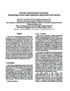
which 39 bags are labeled as positive bags and the other are negative. The number of instances in each bag in MUSK1 is 6 on average, while in MUSK2 the number is more than 60 on average. And the instance in MUSK data sets is defined by a 166-demensional feature vector. For Fox, Tiger, and Elephant data sets from image categorization, each of them contains 100 positive and 100 negative bags, and each instance is a 230dimensional vector. The main goal is to differentiate images containing elephants, tigers and foxes from those that do not, respectively. More information of the data sets can be found in [8]. ELM-MIL network with 166 input units, where each unit corresponds to a dimension of the feature vectors, is trained for ranging hidden units. It should be noted that outputs [0.5, 1] are positive for each unit output, while [0, 0.5] are negative. When applied for multiple instance classification, our method involves two parameters, namely, the regular parameter 𝐶 and the number of hidden neurons. In the experiments, 𝐶 and the number of hidden neurons are selected from {2−3 , 2−2 , 2−1 , 20 , 21 , 22 , 23 , 24 , 25 , 26 , 27 } and {10, 50, 100, 150, 200, 250, 300, 350, 400, 450, 500, 550, 600}, respectively. For comparison with several typical MIL methods, we conduct 10-fold cross validation, which is further repeated 10 times with random different partitions, and the average test accuracy is reported. In Table 1, our method is compared with iterated-discrim APR, Diverse Density, EM-DD, BP-MIP, MI-SVM, C4.5, and Citation-𝑘NN. All the results taken from original literature were obtained via 10-fold cross validation (10CV) except Citation-𝑘NN using leaving one out cross validation (LOO). The values in bracket are the standard deviation and the unavailable results are marked by N/A. The relation between the number of hidden layer nodes and the prediction accuracy with different regulator parameter 𝐶 on MUSK1 and MUSK2 data sets is presented in Figures 1 and 2, respectively. It can be found that when the number of hidden layer is over 300, the accuracy stays at a high level for both MUSK1 and MUSK2. As time is limited, we have conducted experiments on several typical algorithms and recorded their computation time. The training of ELM-MIL, Citation-𝑘NN, BP-MIP, and Diverse Density method are all executed on a 2.6 GHz, i53230 PC, matlab2013b. Since Citation-𝑘NN, Diverse Density, and BP-MIP are all time-consuming algorithms, the time recorded below is based on the total training time of 10CV instead of LOO. The results are shown in Table 2 for MUSK1 and Table 3 for MUSK2. Table 1 suggests that MI-ELM is comparable with stateof-the-art algorithm that is proposed in [13]. Particularly, it can be found from Tables 2 and 3 that the test accuracy of ELM-MIL not only is higher than that of BP-MIP, which is also a multiple instance learning method based on neural network, but also learns significantly faster than that of BPMIP on MUSK data set. Moreover, the iterated-discrim APR algorithm was specially devised for MUSK data, while ELMMIL is a general algorithm. It is clear that, for applicability, ELM-MIL is superior to the APR method. When compared with Citation-𝑘NN, from the point of prediction accuracy, ELM-MIL is worse than Citation-𝑘NN, but from the point
4
Computational Intelligence and Neuroscience Table 1: ELM-MIL performance on benchmark data sets.
Algorithm Iterated-discrim APR [1] Citation-𝑘NN [14] Diverse Density [13] ELM-MIL (proposed) EM-DD [3] BP-MIP [16] MI-SVM [8] C4.5 [15]
MUSK1 92.4 92.4 88 86.5 (4.2) 84.8 83.7 77.9 68.5
MUSK2 89.2 86.3 84 85.8 (4.6) 84.9 80.4 84.3 58.5
Algorithm ELM-MIL Citation-𝑘NN BP-MIP Diverse Density
Prediction accuracy (%)
90 85 80
Tiger N/A N/A N/A 74.6 (2.4) 72.4 N/A 84 N/A
Accuracy 86.5 92.4 83.8 88
Computation time (min) 0.12 1.1 110 350
75
Table 3: Accuracy and computation time on MUSK2.
70 65 60 55
0
100
200 300 400 Number of hidden layer nodes
500
600
C = 0.25 C=4 C = 128
Figure 1: The predictive accuracy of MI-ELM on MUSK1 changes as the number of hidden neurons increases.
MUSK2
95 90 Prediction accuracy (%)
Fox N/A N/A N/A 59.5 (3.7) 56.1 N/A 59.4 N/A
Table 2: Accuracy and computation time on MUSK1.
MUSK1
95
Elephant N/A N/A N/A 76.7 (3.9) 78.3 N/A 81.4 N/A
85
Algorithm ELM-MIL Citation-𝑘NN BP-MIL Diverse Density
Accuracy 85.8 86.3 84 84
Computation time (min) 18 140 1200 3600
of learning time (see Tables 2 and 3) ELM-MIL runs several times faster than Citation-𝑘NN. In addition, ELM-ELM has some advantage compared with other MIL algorithms like Diverse Density, MI-kernel, EM-DD, MI-SVM, C4.5. For example, from Tables 1, 2, and 3, it can be seen that ELM-MIL runs hundreds of times faster than Diverse Density and its performance is also comparable on both Musk1 and Musk2. In addition, both Lozano-Perez’s Diverse Density and EMDD employed some feature selection. Since EM-DD and MIkernel have a mount of parameters to set, it is reasonable to infer that their learning speed is very slow compared with ELM-MIL.
80 75 70 65 60 55 50
0
100
200 300 400 Number of hidden layer nodes
500
600
C = 0.25 C=4 C = 128
Figure 2: The predictive accuracy of MI-ELM on MUSK2 changes as the number of hidden neurons increases.
3.2. Multiple Instance Regression. We compare ELM-MIL, BP-MIP, Diverse Density, and MI-kernel [22] on several multiple instance regression data sets, which are named as LJr.f.s. As for LJ-r.f.s, 𝑟 is the number of relevant features, 𝑓 is the number of features, and 𝑠 is the number of scale factors used for the relevant features indicating the importance of the features. The suffix S suggests that, to partially mimic the MUSK data set, the data set uses only labels that are not near 1/2. Each data set is composed of 92 bags. More information for the regression data sets can be found in [23]. Here four data sets are used, including LJ-160.166.1, LJ160.166.1-S, LJ80.166.1, and LJ-80.166.1-S. And we also perform 10CV tests and report the square loss as well as the computation time in Table 4. Note that the table shows the 10CV results reported in literature, including BP-MIP, Diverse Density, and MI-kernel.
Computational Intelligence and Neuroscience
5
Table 4: Squared loss and computation time (second) on regression data sets. Squared loss Training time MI-Kernel ELM-MIL BP-MIP Diverse Density
LJ-160.166.1 0.00116 0.0376 0.0398 0.0852
90 5.3 4980 12000
LJ-160.166.1-S 0.0127 0.0648 0.0731 0.0052
All of them run on a 2.6 GHz, i5-3230 PC, matlab2013b. Table 4 shows that the square loss of our proposed ELMMIL is worse than MI-kernel, but ELM-MIL takes only tiny mounts of seconds to find appropriate parameters, about twenty times faster than MI-kernel. When compared with BP-MIP and Diverse Density, from the point of performance as well as from the point of training time, ELM-MIL is better than both of them. These results indicate that ELM-MIL is an efficient and effective approach on multiple instance regression task.
4. Conclusions In this paper, a novel multiple instance learning algorithm is proposed based on extreme learning machine. Through modifying the specific error function for the characteristics of multiple instance problems, the most representative instance is chosen in each bag, and the chosen instances are employed to train the extreme learning machine. We have tested ELM-MIL over the benchmark data sets which are taken from applications of drug activity prediction, artificial data sets, and multiple instance regression. Compared with other methods, ELM-MIL algorithm learns much faster and its classification accuracy is slightly worse than stateof-the-art multiple instance algorithms. The experimental results recorded in this paper are rather preliminary. For continuous work, there may be two directions. First, it is possible to improve our method performance by exploiting feature selection techniques [3, 13], that is, feature scaling with Diverse Density and feature reduction with principal component analysis. Next, one can build ensembles of several multiple instance learners to enhance the basic multiple instance learners.
Conflict of Interests The authors declare that there is no conflict of interests regarding the publication of this paper.
Acknowledgments This work was supported by the Specialized Research Fund for the Doctoral Program of Higher Education of China (no. 20124101120001), Key Project for Science and Technology of the Education Department of Henan Province (no. 14A413009), and China Postdoctoral Science Foundation (nos. 2014T70685 and 2013M541992).
8000 45.6 13000 17000
LJ-80.166.1 0.0174 0.0485 0.0487 N/A
120 6.8 5100 N/A
LJ-80.166.1-S 0.0219 0.0748 0.0752 0.1116
10100 42.7 12500 17600
References [1] T. G. Dietterich, R. H. Lathrop, and T. Lozano-P´erez, “Solving the multiple instance problem with axis-parallel rectangles,” Artificial Intelligence, vol. 89, no. 1-2, pp. 31–71, 1997. [2] P. Viola, J. Platt, and C. Zhang, “Multiple instance boosting for object detection,” in Advances in Neural Information Processing Systems, vol. 18, pp. 1417–1426, 2006. [3] Q. Zhang and S. A. Goldman, “EM-DD: an improved multipleinstance learning technique,” in Advances in Neural Information Processing Systems 14, T. G. Dietterich, S. Becker, and Z. Ghahramani, Eds., pp. 1073–1080, MIT Press, Cambridge, Mass, USA, 2002. [4] G. Fung, M. Dundar, B. Krishnapuram, and R. B. Rao, “Multiple instance learning for computer aided diagnosis,” in Advances in Neural Information Processing Systems 19, pp. 425–432, The MIT Press, 2007. [5] C. Leistner, A. Saffari, and H. Bischof, “Miforests: multipleinstance learning with randomized trees,” in Computer Vision— ECCV 2010: 11th European Conference on Computer Vision, Lecture Notes in Computer Science, pp. 29–42, Springer, Berlin, Germany, 2010. [6] Y. Xie, Y. Qu, C. Li, and W. Zhang, “Online multiple instance gradient feature selection for robust visual tracking,” Pattern Recognition Letters, vol. 33, no. 9, pp. 1075–1082, 2012. [7] B. Zeisl, C. Leistner, A. Saffari, and H. Bischof, “On-line semisupervised multiple-instance boosting,” in Proceedings of the IEEE Conference on Computer Vision and Pattern Recognition (CVPR ’10), pp. 1879–1886, IEEE, June 2010. [8] S. Andrews, I. Tsochantaridis, and T. Hofmann, “Support vector machines for multiple instance learning,” in Advances in Neural Information Processing Systems, S. Becker, S. Thrun, and K. Obermayer, Eds., vol. 15, pp. 561–568, MIT Press, Cambridge, Mass, USA, 2003. [9] Z. H. Zhou, Y. Y. Sun, and Y. F. Li, “Multi-instance learning by treating instances as non-I.I.D. samples,” in Proceedings of the 26th International Conference on Machine Learning, L. Bottou and M. Littman, Eds., pp. 1249–1256, Montreal, Canada, June 2009. [10] M. Kim and F. de la Torre, “Multiple instance learning via Gaussian processes,” Data Mining and Knowledge Discovery, vol. 28, no. 4, pp. 1078–1106, 2014. [11] Y. Chen, J. Bi, and J. Z. Wang, “MILES: multiple-instance learning via embedded instance selection,” IEEE Transactions on Pattern Analysis and Machine Intelligence, vol. 28, no. 12, pp. 1931–1947, 2006. [12] Y. Chen and J. Z. Wang, “Image categorization by learning and reasoning with regions,” The Journal of Machine Learning Research, vol. 5, pp. 913–939, 2003/04. [13] O. Maron and T. Lozano-P´erez, “A framework for multipleinstance learning,” in Proceedings of the Conference on Advances
6
[14]
[15]
[16]
[17]
[18]
[19]
[20]
[21]
[22]
[23]
Computational Intelligence and Neuroscience in Neural Information Processing Systems (NIPS ’98), pp. 570– 576, 1998. J. Wang and J.-D. Zucker, “Solving the multiple-instance problem: a lazy learning approach,” in Proceedings of the 17th International Conference on Machine Learning, pp. 1119–1125, San Francisco, Calif, USA, 2000. Y. Chevaleyre and J.-D. Zucker, “Solving multiple-instance and multiple-part learning problems with decision trees and rule sets. application to the mutagenesis problem,” in Advances in Artificial Intelligence, vol. 2056 of Lecture Notes in Computer Science: Lecture Notes in Artificial Intelligence, pp. 204–214, Springer, Berlin, Germany, 2001. Z.-H. Zhou and M.-L. Zhang, “Neural networks for multiinstance learning,” Tech. Rep., AI Lab, Computer Science & Technology Department, Nanjing University, Nanjing, China, 2002. G.-B. Huang, Q.-Y. Zhu, and C.-K. Siew, “Extreme learning machine: a new learning scheme of feedforward neural networks,” in Proceedings of the International Joint Conference on Neural Networks (IJCNN ’04), Budapest, Hungary, July 2004, http://www.ntu.edu.sg/eee/icis/cv/egbhuang.htm. G.-B. Huang, D. H. Wang, and Y. Lan, “Extreme learning machines: a survey,” International Journal of Machine Learning and Cybernetics, vol. 2, no. 2, pp. 107–122, 2011. G.-B. Huang, Q.-Y. Zhu, and C.-K. Siew, “Extreme learning machine: theory and applications,” Neurocomputing, vol. 70, no. 1–3, pp. 489–501, 2006. G.-B. Huang and L. Chen, “Enhanced random search based incremental extreme learning machine,” Neurocomputing, vol. 71, no. 16–18, pp. 3460–3468, 2008. C. Blake, E. Keogh, and C. J. Merz, UCI Repository of Machine Learning Databases, Department of Information and Computer Science, University of California, Irvine, Calif, USA, 1998, http://www.ics.uci.edu/∼mlearn/MLRepository.html. T. Gartner, P. A. Flach, A. Kowalczyk, and A. J. Smola, “Multiinstance kernels,” in Proceedings of the 19th International Conferenceon Machine Learning, pp. 179–186, 2002. R. A. Amar, D. R. Dooly, S. A. Goldman, and Q. Zhang, “Multiple-instance learning of real-valued data,” in Proceedings of the 18th International Conference on Machine Learning, pp. 3–10, 2001.