the TDOA for each microphone pair, and then applying a tracking ... all microphone pairs) by an empirical distribution. ..... 8-channel circular microphone array.
International Workshop on Acoustic Signal Enhancement 2012, 4-6 September 2012, Aachen
A MULTIPLE HYPOTHESIS GAUSSIAN MIXTURE FILTER FOR ACOUSTIC SOURCE LOCALIZATION AND TRACKING Youssef Oualil1,2 , Friedrich Faubel1 and Dietrich Klakow1 1
Spoken Language Systems, Saarland University, Saarbr¨ucken, Germany 2 Idiap Research Institute, CH-1920 Martigny, Switzerland ABSTRACT
In this work, we address the problem of tracking an acoustic source based on measured time differences of arrival (TDOA). The classical solution to this problem consists in using a detector, which estimates the TDOA for each microphone pair, and then applying a tracking algorithm, which integrates the “measured” TDOAs in time. Such a two-stage approach presumes 1) that TDOAs can reliably be estimated; and 2) that errors in detection behave in a well-defined fashion. The presence of noise and reverberation, however, causes larger errors in the TDOA estimates and, thereby, ultimately lowers the tracking performance. We propose to counteract this effect by considering a multiple hypothesis filter, which propagates the TDOA estimation uncertainty to the tracking stage. That is achieved by considering multiple TDOA estimates and then integrating the resulting TDOA observations in the framework of a Gaussian mixture filter. Experimental results show that the proposed filter has a significantly lower angular error than a multiple hypothesis particle filter. Index Terms— Direction of arrival estimation, Microphone Arrays, Monte Carlo methods, Kalman filters 1. INTRODUCTION The problem of TDOA-based source localization can be formulated as a two-stage approach, which consists in first estimating the TDOA that has been introduced at each sensor pair; and then triangulating the source position by integrating the estimated TDOAs in a consistent fashion. While the former is typically performed with the generalized cross correlation (GCC) [1], the latter can elegantly be achieved with a Kalman filter (KF) [2, 3]. Unfortunately, the performance of this approach degrades in the presence of noise and multipath effects, especially under room acoustical conditions where early reflections and reverberation corrupt the GCCs through smearing as well as through the introduction of secondary peaks [4, 5]. This in turn affects the Kalman filter which assumes the error to be a stationary Gaussian process whereas the TDOA error in a multi-path environment is rather time-varying and multimodal. In an attempt to mitigate this problem, Vermaak [5] proposed to use a multiple hypothesis particle filter. This approach has been further improved in [6], where an extended particle filter has been introduced. In this work, we continue along the lines of [5, 6] by proposing a new multiple hypothesis Gaussian mixture filter (MH-GMF), which propagates the uncertainty in the TDOA estimates to the tracking stage. Contrary to previous multiple hypothesis filters, our approach This work was supported by the European Union through the MarieCurie Initial Training Network (ITN) SCALE (Speech Communication with Adaptive LEarning, FP7 grant agreement number 213850); and by the Federal Republic of Germany, through the Cluster of Excellence for Multimodal Computing and Interaction (MMCI).
treats each observation individually, by running a bank of Unscented Kalman filters (UKF). In doing so, the proposed approach incorporates the individual information introduced by each hypothesis. The main problem consists in obtaining the observations. Ideally, we would like to use all possible TDOA combinations from different sensor pairs, weighted with their respective GCC values. As this Cartesian product is computationally intractable, we propose to reduce the number of combinations by first drawing TDOA candidates from the individual GCCs and then combining these TDOAs in a “proximately consistent” fashion. In doing so, we statistically focus on TDOA combinations with high likelihood. In fact, the proposed approach interprets the normalized GCC as a probability density function (pdf) of the TDOA, similar as originally proposed in [5] and firstly applied in [7] for a steered response power (SRP) [4] approach, and then approximates the joint pdf of the TDOA (from all microphone pairs) by an empirical distribution. The angular error of the resulting filter is 69% lower than that of a UKF [2] and up to 35% lower than that of the particle filter approach from [5]. This result was obtained on a real corpus [8], with a quickly moving human speaker in a meeting room. In the remaining part of this paper, we proceed by briefly reviewing the MH-GMF from [9], in Section 2. This is followed by an explanation of how the MH-GMF can be applied to source localization, in Section 3, as well as a presentation of experimental results, in Section 4. 2. MULTIPLE HYPOTHESIS FILTER The problem of tracking a time-varying system state xt based on a sequence y1:t = {y1 , . . . , yt } of corresponding observations is usually formulated as a Bayesian estimation problem in which • Step 1: A process model xt = f (xt−1 , vt ) is used to construct a prior p(xt |y1:t−1 ) for the state estimation problem at time t. • Step 2: The joint predictive distribution p(xt , yt |y1:t−1 ) of state and observation is constructed according to a measurement model yt = h(xt , wt ) with measurement noise wt . • Step 3: The posterior distribution p(xt |y1:t ) is obtained by conditioning the joint predictive density p(xt , yt |y1:t−1 ) on the realized (actually measured) observation Yt = yt . The first step is accomplished by transforming the joint random variable of the last state Xt−1 and process noise Vt according to f : Xt = f (Xt−1 , Vt ). In step 2, the joint distribution of Xt and Yt is constructed by transforming (Xt , Wt ) according to the augmented ˜ [10]: measurement function h � � �� �� �� �� � � Xt Xt xt xt ˜ ˜ =h with h , . Yt Wt wt h(xt , wt )
Both these transformations can generally be performed with the fundamental transformation law of probability. A particularly simple case, however, occurs if f , h are linear and Vt , Wt are Gaussian. In this case, all the involved random variables remain Gaussian at all times and the posterior can be obtained as a conditional Gaussian distribution [10]. This analytical closed form solution is generally known as the Kalman filter. 2.1. Handling Multiple Observations The Kalman filter was designed to receive a single observation yt at time t. In many applied tracking scenarios, however, there are � several (K) potential observation candidates yt = yt1 , . . . , ytK available, some of which may be due to the object of interest, some of which may be due to clutter (noise, reverberation). This problem is typically treated by taking the single most likely observation or by combining multiple observations in a weighted sum, as it is done in the probabilistic data association filter (PDAF) [11]. In [9], we have presented an alternative to these approaches. It treats the multiple observation problem by a) splitting each Kalman filter at time t into K filters; b) assigning each of the resulting filters to one of the observations; and then c) updating them according to the conditioning step (Step 3 in Section 2), as illustrated in Figure 1. In order to integrate the K resulting conditional distributions p(xt |y1:t−1 , ytk ) in one posterior, p(xt |y1:t ) can be written as a marginal distribution of p(xt , k|y1:t ), which, when further expanded under use of p(xt , k|y1:t ) = p(xt |k, y1:t )p(k|y1:t ), gives: p(xt |y1:t ) =
K X
p(xt |ytk , y1:t−1 )p(k|y1:t ) . {z } | k=1
(1)
=p(xt ,k|y1:t )
This is a Gaussian mixture distribution in which the indiviudal posteriors p(xt |ytk , y1:t−1 ) = p(xt |k, y1:t ) constitute Gaussian distributions and in which the p(k|y1:t ) constitute the corresponding weights. The latter can be obtained with Bayes rule: p(k|y1:t ) = PK
p(yt |k, y1:t−1 )γtk
k0 =1
p(yt |k0 , y1:t−1 )γtk
(2)
0
γtk
where = p(k|t) denotes the prior observation probability, which accounts for the confidence or certainty that we put into the k-th observation (similar as motivated in [5]). The p(yt |k, y1:t−1 ) = p(ytk |y1:t−1 ) are observation likelihoods, which can be evaluated by marginalizing the joint predictive distribution p(xt , yt |y1:t−1 ) from step two of the Kalman filter with respect to xt . (c) update
…
KFi
ytK observations
KFi1 (a) split
ω1
+
…
(b) assign
…
yt1
K
KFi
splitting and assigning filters
ωK Gaussian mixture
Fig. 1. Handling multiple observations with a Kalman filter (KFi ).
[9]. As each of the filters is split into K filters at each time t, the number of Gaussian components in general grows exponentially in time. Hence, we reduce the number of mixture components after each iteration by merging Gaussians successively in pairs [9]. Contrary to other tracking frameworks, the MH-GMF treats each observation independently, and assigns weights reflecting the “importance” of the observations in the updated Gaussian mixture. In doing so, this filter allows us to propagate the observations uncertainty to the tracking stage, as well as incorporating the individual information introduced by each observation. In the following, we propose to apply this filter to the acoustic source tracking problem, as we propose a sampling scheme, which captures the uncertainty of the TDOA estimates and propagates it to the tracking stage. We proceed by elaborating on how source localization can be performed with a single KF in Section 3.1 and Section 3.2. Section 3.3 finally presents the multiple observation estimation approach, and how it is integrated into the MH-GMF from Section 2. 3. MH-GMF APPLIED TO SOURCE LOCALIZATION The arrival of sound waves at a microphone array introduces time differences between the individual sensor pairs. This happens in dependence of the angle of arrival – that is, the azimuth θ and elevation φ – as well as the positions mi , i = 1, . . . , M of the microphones. Under the far field assumption, in which the distance of the source from the microphones is neglected, the TDOA at the n-th sensor pair n = {mi , mh } with i 6= h, can be calculated as: τn (d[θ, φ]) =
d[θ, φ]T (mi − mh ) c
(3)
where c denotes the speed of sound and where d[θ, φ] denotes the di� �T rection of arrival cos(φ) sin(θ), cos(φ) cos(θ), sin(φ) . Source localization approaches may use these time differences by either (a) constructing a spatial filter (beamformer), which scans all possible source locations, and then taking that position where the signal energy is maximized [4]. (b) using a two stage approach, which consists in first estimating the TDOAs of all considered microphone pairs and then inferring the most likely source position [2, 3]. 3.1. GCC-Based TDOA Estimation The most popular approach to estimate the TDOA of a microphone pair n = {mi , mh } is the generalized cross-correlation with Phase Transform (PHAT) weighting [1]. This approach is based on calculating the correlation of the signals si (t) and sh (t), which have been received at the microphones, according to: Z 2π Si (ω)Sh∗ (ω) jωτ 1 Rn (τ ) = e dω (4) 2π 0 |Si (ω)Sh∗ (ω)| where Si (ω) and Sh (ω) denote the short-time Fourier transforms of si (t) and sh (t), respectively, and where Rn is their weighted cross correlation. Subsequently, the most “likely” TDOA is extracted as: τbn = argmaxτ Rn (τ )
(5)
2.2. Integration into the Gaussian Mixture Filter Framework After treating the multiple observation problem as proposed above, we have a Gaussian mixture filtering density. This can be handled by maintaining a bank of Kalman filters which are operating in parallel
3.2. Acoustic Source Tracking Based on Estimated TDOAs � Once the TDOA has been estimated for a number of N ≤ M mi2 crophone pairs, source localization can be performed with a Kalman
filter, as described in [2, 3]. In order to do this, we use the following process model for tracking the azimuth θ and elevation φ of the source: � � �� � � � � θt θt−1 θ + vt,θ =f , vt = t−1 (6) φt−1 φt−1 + vt,φ φt where vt,θ and vt,φ denote zero-mean Gaussian process noise with a variance of σθ2 and σφ2 , respectively. Similar to the approaches taken in [2, 3, 5], we use τ1 (d[θt , φt ]) + wt,1 �� � � θt .. yt = h , wt = (7) . φt τN (d[θt , φt ]) + wt,N as a measurement model. In this equation, τn (d[θt , φt ]) denotes the predicted TDOA of the n-th microphone pair, with n = 1, . . . , N , whereas wt,n is zero-mean Gaussian measurement noise with a vari2 ance of σW . This measurement model is nonlinear. Hence the use of an extension of KF is required, we propose to use the UKF, similar as it was originally proposed in [2], but as a single observation filter. 3.3. Applying The Multiple Hypothesis Gaussian Mixture Filter In the Kalman filtering approach from [2, 3], the most likely TDOA is determined individually for each microphone pair. These individual TDOA estimates are subsequently combined to form a joint measurement yt = [ˆ τ1 , . . . , τˆN ]. The error is assumed to follow a Gaussian distribution [2, 3]. This assumption may be true under ideal conditions. In practice, however, the errors in the GCCs (i.e. measurement errors) can be expected to have a multimodal distribution, due to reflections, reverberation and background noise [5]. Hence, we here propose to 1. consider a larger number of observation candidates (hypotheses) ytk with associated confidence weights γtk . 2. process these weighted observations with the multiple hypothesis Gaussian mixture filter (MH-GMF) from Section 2, with the KFs being replaced by UKFs. The aim of this procedure is to propagate the uncertainty from the detection (TDOA estimation) to the tracking stage, by choosing the weighted observation candidates in such a fashion that they capture the observation uncertainty in the GCCs. Let us first consider the observation space Y (does not depend on time), which can be approximated by the Cartesian product of all possible TDOAs from N different microphone pairs : n o N Y = y 1 , . . . , y K , × {−τnmax , . . . , τnmax } (8) n=1
� � k where y k = τ1k , . . . , τN with k = 1, . . . , K. τnmax denotes the maximum TDOA of microphone pair n and K is the cardinality of Y. Then, interpreting the GCC as a likelihood function (as done in [7] for the SRP) and further assuming that errors in the GCCs are statistically independent [5], the confidence or prior observation likelihood of a particular combination y k can be calculated as the product of the individual GCC values Rn (τnk ): γtk =
N Y
˜ n (τnk ) with R ˜ n (τ ) , P Rn (τ ) R 0 τ 0 Rn (τ ) n=1
(9)
P where the division by τ 0 Rn (τ 0 ) normalizes the total probability to 1. This gives us the following observation density:
pmeasured (yt ) =
K X
� � γtk δ yt − y k
(10)
k=1
where the y k and γtk are given by (8) and (9), respectively. As a next step, we could now pass this density to the multiple hypothesis filter from Section 2. But, the fact that the Cartesian prodQconsidering max + 1) different combinations, this uct results in K = N n=1 (2τn approach has to be dismissed as intractable. Hence, we reduce the number of observations by approximating (10) through a sampling scheme, which samples observations from high likelihood regions of the observation space. 0
Sampling from the GCCs: In order to obtain a set {yt1 , . . . , ytK } of K 0