Efficient Gaussian Mixture Filter for Hybrid Positioning

Proceedings of PLANS 2008 IEEE/ION Position Location and Navigation Symposium Pages 60-66

Efficient Gaussian Mixture Filter for Hybrid Positioning Simo Ali-Löytty Department of Mathematics Tampere University of Technology Finland

Abstract—This paper presents a new way to apply Gaussian Mixture Filter (GMF) to hybrid positioning. The idea of this new GMF (Efficient Gaussian Mixture Filter, EGMF) is to split the state space into pieces using parallel planes and approximate posterior in every piece as Gaussian. EGMF outperforms the traditional single-component positioning filters, for example the Extended Kalman Filter and the Unscented Kalman Filter, in nonlinear hybrid positioning. Furthermore, EGMF has some advantages with respect to other GMF variants, for example EGMF gives the same or better performance than the Sigma Point Gaussian Mixture (SPGM) [1] with a smaller number of mixture components, i.e. smaller computational and memory requirements. If we consider only one time step, EGMF gives optimal results in the linear case, in the sense of mean and covariance, whereas other GMFs gives suboptimal results.

I. I NTRODUCTION Positioning filters, such as GMF [2]–[4], are used to compute an estimate of the state using current and past measurement data. Usually, the mean of the posterior distribution is this estimate. A consistent filter also provides correct information on the accuracy of its state estimate, e.g. in the form of an estimated error covariance. Generally, GMF is a filter whose approximate prior and posterior densities are Gaussian Mixtures (GMs), a linear combination of Gaussian densities where weights are between 0 and 1. GMF is an extension of Kalman type filters. In particular, The Extended Kalman Filter (EKF) [5]–[8], Second Order Extended Kalman Filter (EKF2) [5], [6], [9], Unscented Kalman Filters (UKF) [10] and a bank of these filters, are special cases of GMF. Hybrid positioning means that measurements used in positioning come from many different sources e.g. Global Navigation Satellite System, Inertial Measurement Unit, or local wireless networks such as a cellular network. Range, pseudorange, delta range, altitude, base station sector and compass measurements are examples of typical measurements in hybrid positioning. In the hybrid positioning case, it is usual that measurements are nonlinear and because of that posterior density may have multiple peaks (multiple positioning solutions). In these cases, traditional single-component positioning filters, such as EKF, do not give good performance [9]. This is the reason for developing GMF for hybrid positioning [1]. Other possibility is to use a general nonlinear Bayesian filter, which is usually implemented as a particle filter or a point mass filter. These filters usually work correctly and give good positioning accuracy but require much computation time and memory.

An outline of the paper is as follows. In Section II, we glance at Bayesian filtering. In Section III, we study the basics of the GM and of the GMF. In Section IV, we present the new method, box GM approximation, to approximate Gaussian as GM. In Section V we apply the box GM approximation to the filtering framework and get the Box Gaussian Mixture Filter (BGMF). In Section V we also present Sigma Point Gaussian Mixture Filter (SPGMF) [1]. In Section VI, we develop BGMF so that it gives exact mean and covariance in one step linear case. We call that new filter the Efficient Gaussian Mixture Filter (EGMF). In Section VII, we compute one step comparison of EKF, SPGMF, BGMF and EGMF. Finally in Section VIII, we present simulation results where we compare different GMFs and a bootstrap particle filter [11]. II. BAYESIAN F ILTERING We consider the discrete-time non-linear non-Gaussian system xk = fk−1 (xk−1 ) + wk−1 ,

(1)

yk = hk (xk ) + vk ,

(2)

where the vectors xk ∈ Rnx and yk ∈ Rnyk represent the state of the system and the measurement at time tk , k ∈ N, respectively. We assume that errors wk and vk are white, mutually independent and independent of the initial state x0 . We denote the density functions of wk and vk by pwk and pvk , respectively. The aim of filtering is to find the conditional probability density function (posterior) p(xk |y1:k ), △

where y1:k = y1 , . . . , yk are past and current measurements. The posterior can be determined recursively according to the following relations. Prediction (prior): Z p(xk |y1:k−1 ) = p(xk |xk−1 )p(xk−1 |y1:k−1 )dxk−1 ; (3) Update (posterior): p(xk |y1:k ) = R

p(yk |xk )p(xk |y1:k−1 ) , p(yk |xk )p(xk |y1:k−1 )dxk

where the transition pdf is

p(xk |xk−1 ) = pwk−1 (xk − fk−1 (xk−1 ))

(4)

and the likelihood p(yk |xk ) = pvk (yk − hk (xk )). The initial condition for the recursion is given by the pdf of the initial state p(x0 |y1:0 ) = p(x0 ). Knowledge of the posterior distribution (4) enables one to compute an optimal state estimate with respect to any criterion. For example, the minimum mean-square error (MMSE) estimate is the conditional mean of xk [5], [12]. In general and in our case, the conditional probability density function cannot be determined analytically. III. G AUSSIAN M IXTURE F ILTER A. Gaussian Mixture Definition 1 (Gaussian Mixture): an n-dimensional random variable x is N -component Gaussian Mixture (GM) if its characteristic function has the form N X 1 αj exp itT µj − tT Σj t , ϕx (t) = (5) 2 j=1 where µj ∈ Rn , Σj ∈ Rn×n is symmetric positive semidefinite PN (Σj ≥ 0), αj ≥ 0 and j=1 αj = 1. We use the abbreviation x ∼ M(αj , µj , Σj )(j) . If random variable x is GM, x ∼ M(αj , µj , Σj )(j) and all matrices Σj are symmetric positive definite (Σj > 0), then x has a density function px (ξ) =

N X

µ αj NΣjj (x),

(6)

j=1

µ NΣjj (x)

is the Gaussian density function with mean µj where and covariance Σj T −1 1 1 µ NΣjj (x) = e− 2 (x−µj ) Σj (x−µj ) . np (2π) 2 det Σj is

Theorem 3: Let random variables x ∼ M(αj , µj , Σj )(j) and v ∼ N(0, R) be independent. Define y = Hx + v, where H ∈ Rm×n . Then y ∼ M(αj , Hµj , HΣj HT + R)(j) . Proof: Because x and v are independent then Hx and v are also independent. Futhermore, Ind.

ϕHx+v (t) = ϕHx (t)ϕv (t) = ϕx (HT t)ϕv (t) N 1 1 (5) X αi exp itT Hµj − tT HΣj HT t exp − tT Rt = 2 2 j=1 N X 1 αj exp itT Hµj − tT HΣj HT + R t . = 2 j=1

B. Gaussian Mixture Filter GMF is (an approximation of) the Bayesian Filter (see Section II). The idea of GMF [2]–[4] (also called Gaussian Sum Filter) is that both prior density (3) and posterior density (4) are GMs. Algorithm 1 Linearized GMF + + Initial state at time t0 : x0 ∼ M(α+ j,0 , xj,0 , Pj,0 )(j) for k = 1 to n do 1) Prediction step, prior at time tk (see Thm. 3): − − M(α− j,k , xj,k , Pj,k )(j) ,

Theorem 2: Let x ∼ M(αj , µj , Σj )(j) . Then the mean of x E(x) =

N X

2)

αj µj ,

j=1

and the covariance of x is N X αj Σj + (µj − E(x))(µj − E(x))T . V(x) =

3)

+ + M(α+ j,k , xj,k , Pj,k )(j) ,

where

j=1

hk (¯ xj,k )+Hj,k (x− −¯ xj,k ) j,k

− α+ j,k ∝ αj,k NH

Proof: Using the properties of characteristic function [13], we get X 1 ′ T αj µj (ϕx (t)|t=0 ) = i j=1

and V(x) = −ϕ′′x (t)|t=0 − E(x) E(x)T =

N X j=1

=

N X j=1

αj (µj µTj + Σj ) − E(x) E(x)T αj Σj + (µj − E(x))(µj − E(x))T .

(y )

− k T j,k Pj,k Hj,k +Rk − = xj,k +Kj,k (yk −hk (¯ xj,k )−Hj,k (x− ¯j,k )) j,k − x − = (I − Kj,k Hj,k )Pj,k − T T −1 Kj,k = P− j,k Hj,k (Hj,k Pj,k Hj,k + Rk ) ∂hk (x) and x ¯j,k are selected Here Hj,k = ∂x x=¯ xj,k linearization points, e.g. in EKF x ¯j,k = x− j,k .

x+ j,k P+ j,k

N

E(x) =

where + α− j,k = αj,k−1 + x− j,k = Fk−1 xj,k−1 − T Pj,k = Fk−1 P+ j,k−1 Fk−1 + Qk−1 Approximate selected components as GM (see Section IV) Update step, posterior at time tk [14]:

4)

Reduce number of components: forgetting, merging and resampling [2], [15], [16]. end for Algorithm 1 presents one version of GMF, Linearized GMF. Algorithm 1 uses the following assumptions:

1) Initial state x0 is non-singular GM, which means that x0 has density function (6). 2) State model (1) is linear

where index j = 1, . . . , nbox , and parameters are Z px (ξ)dξ = Φ (lj ) − Φ (lj−1 ) , αj = Aj

xk = Fk−1 xk−1 + wk−1 . 3) Errors wk ∼ N(0, Qk ) and vk ∼ N(0, Rk ) and Rk is non-singular. Note that it is straightforward to extend Linearized GMF to cases where also the errors wk and vk are GMs. IV. A PPROXIMATE G AUSSIAN

AS

G AUSSIAN M IXTURE

As we know, EKF in hybrid positioning [9] has a consistency problem. The key reason for inconsistency is nonlinearity. Now we assume that we have only one measurement and our prior is Gaussian x ∼ N(ˆ x, P). The application to the general case is given in Section V. One measure of nonlinearity is [1], [6], [9] r tr(He PHe P) (7) N onlinearity = − 1, R where He is Hessian matrix of scalar measurement h(x), R is a covariance of measurement error and P is a covariance of the state component. One possibility to overcome the nonlinearity problem (i.e. minimize N onlinearity (7)) is to approximate Gaussian as GM whose components have smaller covariance matrices than the orginal Gaussian. One method for doing so is the Sigma Point Gaussian Mixture (SPGM) [1] (see Section IV-A). One drawback of SPGM is that SPGM splits one Gaussian to 2nx + 1 components GM, regardless of our measurement equation and Hessian matrix He . Because of this, we present a new method of approximating Gaussian as GM (see Section IV-B). We call this method as a Box GM, because it has connection to the ”Box”-method [17].

The SPGM is given on Table I. SPGM has the same mean, covariance, and third moments as the original Gaussian distribution x ∼ N(ˆ x, P) [1]. TABLE I SPGM M(αj , µj , Σj )(j)

APPROXIMATION OF G AUSSIAN x PARAMETERS τ ∈ (0, 1) AND κ > 0.

Index j 0 1, . . . , nx nx + 1, . . . , 2nx

αj κ κ+nx 1 2(κ+nx ) 1 2(κ+nx )

∼ N(ˆ x, P),

µj

Σj

x ˆ √ √ x ˆ + τ κ + nx Pej √ √ x ˆ − τ κ + nx Pej−n

(1 − τ 2 )P (1 − τ 2 )P (1 − τ 2 )P

B. Box GM approximation The idea of the Box GM approximation is that we split the state space using parallel planes and approximate the Gaussian inside every piece with one GM component using moment matching method. The Box GM approximation of the Gaussian x ∼ N(ˆ x, P), with P > 0, is xN ∼ M(αj , µj , Σj )(j) ,

(8)

l2 j

where Φ is the standard normal cumulative density function and sets Aj have the following form Aj = x lj < aT (x − xˆ) ≤ lj+1 ,

where aT Pa = 1 and vector l is monotonic increasing so that l1 = −∞ and lnbox +1 = ∞ so these sets constitute a partition of Rnx . 1) Mean and covariance of the Box GM approximation: In this Section, we compute the mean and the covariance of the GM approximation xN Eq. (8). First of all, because Σj > 0 ∀j, αj > 0 ∀j and Z nbox nbox Z X X αj = px (ξ)dξ = px (ξ)dξ = 1, j=1

j=1

Aj

then xN is a valid GM. The mean of xN is nbox Z nbox X X T hm. 2 αj µj = ξpx (ξ)dξ = xˆ. E (xN ) = j=1

j=1

Aj

The covariance of xN is V (xN )

A. Sigma Point GM approximation

l2 j−1

px (ξ) e− 2 − e− 2 √ ξ µj = , dξ = x ˆ + Paǫj , ǫj = αj 2παj Aj Z px (ξ) (ξ − µj )(ξ − µj )T Σj = dξ αj Aj   l2 l2 − 2j − j−1 2 lj e −l e √ j−1 = P − Pa  + ǫ2j  aT P. 2παj Z

T hm. 2

=

nbox X j=1

=

nbox Z X j=1

Aj

αj (µj µTj + Σj ) − x ˆxˆT

ξξ T px (ξ)dξ − x ˆx ˆT = P.

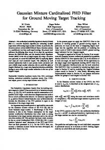
So the mean and the covariance of the GM approximation are the same as the mean and the covariance of the ordinary Gaussian. Because of this, we can say that Box GM approximation is a moment matching method. 2) Contour plot of the Box GM approximation: In Fig. 1 we compare the density function of the Gaussian distribution 0 13 −12 x∼N , . (9) 0 −12 13 and the density function of its approximation by a Box GM 0.2774 with parameters a ≈ and 0 l = −∞ −1.28 1.28 ∞ 0 0.1 0.9 1 ≈ Φ−1 .

Fig. 1 shows the contour plots of the Gaussian and the Box GM density functions so that 50% of probability is inside the

Gaussian Box GM

o n T T i , where ai Pi ai = 1 ∀i, Aij = x lji < ai (x − xî ) ≤ lj+1 i i vectors l are monotonic increasing so that l1 = −∞ and lni i +1 = ∞. So for all i sets Aij constitute a partition of Rnx . BGMF (see Section V) approximates µi

i

χAij (x) NxPˆ i (x) ≈ αij NΣji (x) and j 0 0 NR (y − h(x)) ≈ NR y − h(µij ) − Hµij (x − µij )

0.5 Planes

0.95

Fig. 1. Contour plot example of the Box GM, when approximating density is Gaussian Eq. (9)

innermost curve and 95% of probability is inside the outermost curve. We see that the density function of the Box GM is quite good approximation of the Gaussian density function Eq. (9). V. B OX G AUSSIAN M IXTURE F ILTER AND S IGMA P OINT G AUSSIAN M IXTURE F ILTER Box Gaussian Mixture Filter (BGMF) is a straightforward application of the Box GM approximation to the Gaussian Mixture filtering framework. BGMF is a Linearized GMF (see Alg. 1), where the step 2 is the following. First we compute N onlinearity (7) statistics for every component and measurement. We select the components that have at least one highly nonlinear measurement with N onlinearity > 0. Every selected component we replace by its Box GM approximation (Section IV-B). The SPGMF, which is presented in the paper [1] with name GMFekf S , is also a Linearized GMF (see Alg. 1) and almost the same as BGMF. Only difference between SPGMF and BGMF is that SPGM approximates selected Gaussians using SPGM approximation (see Table I), while BGMF uses the Box GM approximation (Section IV-B). VI. E FFICIENT G AUSSIAN M IXTURE F ILTER In this Section, we derive a new GMF, Efficient Gaussian Mixture Filter (EGMF). Prediction step (Eq. (3)) of EGMF is the same as prediction step of Linearized GMF (see Alg. 1). Now we consider update step (Eq. (4)). Assume that prior distribution is a GM x ∼ M(β i , xî , Pi )(i)

where αij , µij and Σij are computed using the Box GM algorithm (see Section IV-B) and Hµij = h′ (µij ). So BGMF approximates both prior and likelihood before multiplying them. EGMF first approximates the likelihood as N0R (y − h(x)) ≈ N0R y − h(µij ) − Hµij (x − µij ) and then multiplies it with the prior: p(x|y) ∝ nprior ni i ⋆ X iX χAij (x) NxPˆ i (x) N0R y − h(µij ) − Hµij (x − µij ) β ≈ j=1

i=1 nprior

=

X i=1

βi

ni X

x î

χAij (x)γji NPji (x) j

j=1

(10) where xi −µij ) h(µij )+Hµi (ˆ

γji = NH

P µi j

j i HT +R µi j

xîj = x î + Kij (y − h(µij ) − Hµij (ˆ xi − µij )) Pij = (I − Kij Hµij )Pi Kij = Pi HTµi (Hµij Pi HTµi + R)−1 . j

j

Note that ⋆ approximation is exact if h(x) is linear. Then we use the Box GM algorithm (see Section IV-B) and get ⋆

p(x|y) ∝ ≈ =

and measurement model is (see (2)) y = h(x) + v, where v ∼ N(0, R). Now the posterior density function is nprior

p(x|y) ∝ nprior

=

X i=1

βi

X

i=1 ni X j=1

i

β i NxPˆ i (x) N0R (y − h(x)) i

χAij (x) NxPˆ i (x) N0R (y − h(x)) ,

(y)

≈

nprior

X

βi

ni X

x î

χAij (x)γji NPji (x) j

j=1 i=1 nprior ni XX x î β i γji χBji (x) NPji (x) j i=1 j=1 nprior ni XX µ ¯i α ¯ ij β i γji NΣ¯ji (x) j i=1 j=1

(11)

¯ i are computed using the Box GM where α ¯ ij , µ ¯ij and Σ j algorithm, when we noted that o n T îj ) ≤ mij+1 Bji = x mij < bi (x − x o n T i = Aij , î ) ≤ lj+1 = x lji < ai (x − x

Mahalanobis distance 4

Lissack−Fu distance EKF SPGMF BGMF EGMF Nonlinearity

3

2

EKF SPGMF BGMF EGMF Nonlinearity

1

2

1

0 100

500 1000 1500 Distance between prior mean and base station

0 100

500 1000 1500 Distance between prior mean and base station

Fig. 2. Mahalanobis distance between exact mean and mean approximations. Significance of nonlinearity (see equation (7)) is also shown.

Fig. 3. Lissack-Fu distance between exact posterior and posterior approximations. Significance of nonlinearity (see equation (7)) is also shown.

where

with 5002 points [18]. Approximation of the exact density function is computed using EKF, SPGMF, BGMF and EGMF. The SPGMF uses parameters κ =4 and τ = 12 and the BGMF 0 and EGMF uses parameters a = and 1

ai T ⇒ bi Pij bi = 1 bi = q T ai Pij ai T

li + ai (ˆ xi − x îj ) q m = ⇒ mij < mij+1 ∀j , ai T Pij ai i

mi1 = −∞ and mini = ∞.

Now we get that the posterior of EGMF is Pnprior Pni i i i µ¯ij ¯j β γj NΣ¯ i (x) i=1 j=1 α Pnprior Pni i i ij p(x|y) ≈ . ¯ j β γj i=1 j=1 α

If we consider the linear case and only one time step, EGMF gives a correct mean and a correct covariance, because linearity ensures that ⋆ approximation in Eq. (10) is exact and the Box GM approximation maintains the mean and the covariance in Eq. (11) (see Section IV-B1). SPGMF and BGMF can give a wrong mean and a wrong covariance in one time step linear case. VII. O NE STEP COMPARISON OF EKF, SPGMF, BGMF AND EGMF

This is the same example as in paper [1], but we have included BGMF (Section V) and EGMF (Section VI) to this example. This example presents a comparison between EKF posterior, SPGMF (Section V) posterior, BGMF posterior and EGMF posterior, when prior distribution is d 1002 0 x∼N , , 0 0 3002 and we get one base station range measurement (2), where y = 1000, h(x) = kxk and v ∼ N(0, 1002 ). The base station is located in origin and so d is the distance between prior mean and the base station. ”Exact” posterior density function pexact (x) is computed using a point-mass filter,

300

−∞ −1.28 1.28 ∞ 0 0.1 0.9 1 ≈ Φ−1 .

l=

Note that both BGMF and EGMF have only three GM components whereas SPGMF has five GM components. Comparison between EKF, SPGMF, BGMF and EGMF contains two parts. First we compute the Mahalanobis distance between the mean of the exact posterior mean and means of approximations q (µexact − µapp )T Σ−1 exact (µexact − µapp ). These results are shown in Fig. 2. The value of the Nonlinearity function (7) is also plotted in Fig. 2. We see that Mahalanobis distance between EKF mean and exact mean increases rapidly when nonlinearity becomes more significant. In that case SPGMF, BGMF and EGMF give much better results than EKF. EGMF has the same or smaller Mahalanobis distance than BGMF. Furthermore, SPGMF, BGMF and EGMF give always as good results as EKF even when there is no significant nonlinearity. Second, we compute the first order Lissack-Fu distance Z |pexact (x) − papp (x)|dx, between exact posterior and the approximations (also called a total variation norm). These results are in Fig. 3. The value of the Nonlinearity function (7) is also plotted. We see that SPGMF, BGMF and EGMF give smaller Lissack-Fu distance than EKF. Difference between EGMF Lissack-Fu distance and EKF Lissack-Fu distance increases when nonlinearity becomes more significant. EKF Lissack-Fu distance is almost 2 (maximum value) when d = 100, so the exact posterior and the EKF posterior approximation are almost totally separate.

Furthermore, EGMF has Lissack-Fu distance same as or smaller than BGMF. Overall SPGMF, BGMF and EGMF work almost identically although EGMF and BGMF use only three mixture component versus five SPGMF mixture components. In this example, EGMF gives the best results compared to the other filters. Furthermore SPGMF, BGMF and EGMF all give much better results than EKF when nonlinearity is significant. VIII. S IMULATIONS In the simulations, we use the position-velocity model, so ru consists of user position vector ru and the state x = vu user velocity vector vu , which are in East-North-Up (ENU) coordinate system. In this model the user velocity is a random walk process [19]. Now the state-dynamic (1) is xk = Φk−1 xk−1 + wk−1 , where Φk−1 =

I ∆tk I 0 I

,

∆tk = tk − tk−1 , and wk−1 is white, zero mean and Gaussian noise, with covariance  ∆t3 σ2  ∆t2k σp2 k p I 0 I 0 3 2  ∆t3k σa2 ∆t2k σa2    0 0 3 2  , Qk−1 =  ∆t2 σ2  ∆tk σp2 k p   I 0 I 0 2 1 0

∆t2k σa2 2

0

∆tk σa2 1

2

where σp2 = 2 ms3 represents the velocity errors on the East2 North plane and σa2 = 0.01 ms3 represents the velocity errors in the vertical direction. [9], [20] In our simulations, we use base station range measurements, altitude measurements, satellite pseudorange measurements and satellite delta range measurements (see Eq. (2)). y b = krb − ru k + ǫb , y a = 0 0 1 ru + ǫa ,

y s = krs − ru k + b + ǫs , (rs − ru )T (vs − vu ) + b˙ + ǫ˙s , y˙ s = krs − ru k

where rb is a base station position vector, rs is a satellite position vector, b is clock bias, vs is a satellite velocity vector, b˙ is clock drift and ǫ:s are error terms. We use satellite measurements only when there is more than one satellite measurement available, so that bias can be eliminated. These are the same measurements equations as in the papers [1], [15], [17]. Simulations are made using Personal Navigation Filter Framework (PNaFF) [21]. PNaFF is a comprehensive simulation and filtering test bench that we are developing and using in the Personal Positioning Algorithms Research Group. PNaFF uses Earth Centered Earth Fixed (ECEF) coordinate system so we have converted our models from ENU to ECEF.

A

SUMMARY OF

TABLE II 200 DIFFERENT SIMULATIONS WITH BASE STATION MEASUREMENTS .

Solver EKFno res. EKF EKF2 UKF SPGMF PF2500 BGMF EGMF Ref

Time ∝ 4 10 11 23 62 38 32 32 ∞

Err. rms 284 236 214 213 210 201 194 191 155

Err. 95% 622 465 433 421 399 397 371 360 287

Err. ref 127 83 65 58 69 73 58 57 0

Inc. % 9.9 6.6 2.8 2.3 3.3 21.9 2.8 2.8 0.1

A. Summary of base station cases On Table II, we have listed a summary of two hundred 120 second simulations, which use only base station measurements. This means that simulations use base station range measurements with variance (80 m)2 , very inaccurate altitude measurements with variance (300 m)2 and restrictive information. Restrictive information is in our case base station 120◦-sector and maximum range information. So when we have restrictive information we know that user is inside the particular area, which is restricted using sector and maximum range information. Restrictive information are used in the same way as in paper [17]. Summary consist of following columns: Time is computation time using Matlab in our implementation, scaled so that computation time of EKF is 10. This gives a rough idea of the relative time complexity of each algorithm. Err. rms is 3D root mean square position error. Err. 95% gives a radius containing 95 % of the 3D errors. Err. ref. is 3D error to reference posterior mean, which is computed using a particle filter with systematic resampling and 106 particles [11]. Inc. % is a percentage of time where the filter is inconsistent with respect to the general inconsistency test, with risk level 5% [9]. Solvers are sorted so that rms errors are in descending order. PFN indicates particle filter with systematic resampling and N particles [11], so reference solution is the same as PF106 . On these simulations BGMF splits, when highly nonlinearity exists, one GM component into four components with equal weights. In that case the parameter l of the Box GM approximation (see Section IV-B) is 0 14 12 34 1 l = Φ−1 . EGMF also uses the same l parameter (see Section VI). In Table II, the results are the realization of random variables and if we run these simulations again we possibly get a slightly different result. The following conclusions can be drawn based on simulations and theory. • Both BGMF and EGMF give a better result (in all listed criteria) than SPGMF or PF2500 • Computation time of BGMF and EGMF is approximately half of computation time of SPGMF. • EGMF gives much better results than traditional EKF (EKFno res. ).

A

SUMMARY OF

TABLE III 1000 DIFFERENT SIMULATIONS WITH BASE STATION AND SATELLITE MEASUREMENTS .

Solver EKFno res. EKF UKF SPGMF PF2500 EKF2 BGMF EGMF Ref

•

Time ∝ 6 10 28 38 43 11 20 20 ∞

Err. rms 115 101 95 95 95 94 93 92 83

Err. 95% 215 184 174 173 160 176 170 169 156

Err. ref 23 16 11 13 12 12 12 12 0

Inc. % 3.0 2.1 1.1 1.2 1.8 1.2 1.0 1.0 1.2

PF2500 has a serious inconsistency problem, i.e. it under estimates the state covariance.

B. Summary of mixed cases In Table III, we have listed a summary of one thousand 120 second simulations, which use both base station and satellite measurements with varying parameters. Parameters are following: variance of base station range measurement = (30 m)2 , variance of satellite pseudorange measurement ≈ (3 m)2 and variance of delta range measurement ≈ (0.1 ms )2 . We use restrictive information in the same way as simulations on Section VIII-A. Also notations and filters are the same as simulations on Section VIII-A. The following conclusions can be drawn based on simulations. • Order of filter in Table III is almost the same as in Table II. • Differences between different filters are smaller than in Table II, because there are also satellite measurements (very accurate linear measurements). • Computation time of BGMF and EGMF is approximately half of computation time of SPGMF. • EGMF gives much better results than traditional EKF (EKFno res. ). IX. C ONCLUSION In this article, we have presented two new Gaussian Mixture Filters for the hybrid positioning: the Box GMF and the Efficient GMF. BGMF and EGMF are almost the same filter, because of this their performances are almost the same. Nevertheless EGMF gives slightly better results than BGMF. Both filters outperform the Sigma Point GMF, which outperforms the traditional single-component Kalman type filters such as EKF, UKF and EKF2. EGMF and BGMF also outperform particle filter, when number of particles is selected so that particle filter uses about the same time of computation as EGMF. GMFs and EKF works equivalently if we have only linear measurements, but the more nonlinearity occurs the better result GMFs give compared to EKF.

ACKNOWLEDGMENT The author would like to thank Niilo Sirola and Robert Piché for their comments and suggestions. This study was partly funded by Nokia Corporation. The author acknowledges the financial support of the Nokia Foundation and the Tampere Graduate School in Information Science and Engineering. R EFERENCES [1] S. Ali-Löytty and N. Sirola, “Gaussian mixture filter and hybrid positioning,” in Proceedings of ION GNSS 2007, Fort Worth, Texas, Fort Worth, September 2007, pp. 562–570. [2] H. W. Sorenson and D. L. Alspach, “Recursive Bayesian estimation using Gaussian sums,” Automatica, vol. 7, no. 4, pp. 465–479, July 1971. [3] D. L. Alspach and H. W. Sorenson, “Nonlinear Bayesian estimation using Gaussian sum approximations,” IEEE Transactions on Automatic Control, vol. 17, no. 4, pp. 439–448, Aug 1972. [4] B. D. O. Anderson and J. B. Moore, Optimal Filtering, ser. Electrical Engineering, T. Kailath, Ed. Prentice-Hall, Inc., 1979. [5] Y. Bar-Shalom, R. X. Li, and T. Kirubarajan, Estimation with Applications to Tracking and Navigation, Theory Algorithms and Software. John Wiley & Sons, 2001. [6] A. H. Jazwinski, Stochastic Processes and Filtering Theory, ser. Mathematics in Science and Engineering. Academic Press, 1970, vol. 64. [7] C. Ma, “Integration of GPS and cellular networks to improve wireless location performance,” Proceedings of ION GPS/GNSS 2003, pp. 1585– 1596, 2003. [8] G. Heinrichs, F. Dovis, M. Gianola, and P. Mulassano, “Navigation and communication hybrid positioning with a common receiver architecture,” Proceedings of The European Navigation Conference GNSS 2004, 2004. [9] S. Ali-Löytty, N. Sirola, and R. Piché, “Consistency of three Kalman filter extensions in hybrid navigation,” in Proceedings of The European Navigation Conference GNSS 2005, Munich, Germany, Jul. 2005. [10] S. J. Julier, J. K. Uhlmann, and H. F. Durrant-Whyte, “A new approach for filtering nonlinear systems,” in American Control Conference, vol. 3, 1995, pp. 1628–1632. [11] M. S. Arulampalam, S. Maskell, N. Gordon, and T. Clapp, “A tutorial on particle filters for online nonlinear/non-Gaussian Bayesian tracking,” IEEE Transactions on Signal Processing, vol. 50, no. 2, pp. 174–188, 2002. [12] B. Ristic, S. Arulampalam, and N. Gordon, Beyond the Kalman Filter, Particle Filters for Tracking Applications. Boston, London: Artech House, 2004. [13] K. V. Mardia, J. T. Kent, and J. M. Bibby, Multivariate analysis, ser. Probability and mathematical statistics. London Academic Press, 1989. [14] M. S. Grewal and A. P. Andrews, Kalman Filtering, Theory and Practice, ser. Prentice hall information and system sciences. Prentice-Hall, Inc., 1993. [15] S. Ali-Löytty and N. Sirola, “Gaussian mixture filter in hybrid navigation,” in Proceedings of The European Navigation Conference GNSS 2007, 2007. [16] D. J. Salmond, “Mixture reduction algorithms for target tracking,” State Estimation in Aerospace and Tracking Applications, IEE Colloquium on, pp. 7/1–7/4, 1989. [17] S. Ali-Löytty and N. Sirola, “A modified Kalman filter for hybrid positioning,” in Proceedings of ION GNSS 2006, September 2006. [18] R. S. Bucy and K. D. Senne, “Digital synthesis of non-linear filters,” Automatica, vol. 7, no. 3, pp. 287–298, May 1971. [19] R. G. Brown, Introduction to Random Signal Analysis and Kalman Filtering. John Wiley & Sons, 1983. [20] P. S. Maybeck, Stochastic Models, Estimation, and Control, ser. Mathematics in Science and Engineering. Academic Press, 1979, vol. 141. [21] M. Raitoharju, N. Sirola, S. Ali-Löytty, and R. Piché, “PNaFF: a modular software platform for testing hybrid positioning estimation algorithms,” in WPNC08 Workshop on Positioning, Navigation and Communication, Hannover, 28 Mar 2008, 2008, (accepted). [Online]. Available: http://www.wpnc.net/