A Multiscale Modeling of Multiple Physics

March 6, 2013

15:5

PSP Book - 9in x 6in

Chapter 17

A Multiscale Modeling of Multiple Physics Xianqiao Wang,a Jiaoyan Li,a James D. Lee,a and Azim Eskandarianb a Department of Mechanical and Aerospace Engineering,

The George Washington University,

801 22nd Street, NW Washington, DC 20052, USA

b Department of Civil and Environmental Engineering,

The George Washington University,

801 22nd Street, NW Washington, DC 20052, USA

[email protected]

Many complex materials require multiscale and/or multiphysics research to connect structure to properties and ultimately to function. The unique amalgamation of the discrete multiple length spectrum and its multiple physics principles creates a unprece dented area whose evolution can only be unveiled through the marriage of advancement of theoretical studies, exploitation of com putational methods, and non-traditional experimental validation. This chapter presents a coarse-grained molecular dynamics (CG MD) simulation method coupling with thermal, mechanical and electrical mechanism, aiming at a seamless transition from the atomistic to the continuum description of multi-element crystalline solids (which has more than one kind of atom in the unit cell). By

Handbook of Micromechanics and Nanomechanics Edited by Shaofan Li and Xin-Lin Gao c 2013 Pan Stanford Publishing Pte. Ltd. Copyright � ISBN 978-981-4411-23-3 (Hardcover), 978-981-4411-24-0 (eBook) www.panstanford.com

© 2013 by Taylor & Francis Group, LLC

17-Shaofan-Li-c17

March 6, 2013

15:5


Downloaded by [Virginia Commonwealth University (VIVA)] at 13:59 23 June 2015

620 A Multiscale Modeling of Multiple Physics

accounting for the upgraded Nosé–Hoover thermostat and Lorentz force, we put forth a novel way to appreciate the full benefit of coupling the thermal, mechanical and electromagnetic fields at nano/micro scale. Contrary to many multiscale approaches, the CG-MD simulation method proposed here is naturally suitable for the multiphysics analysis of multi-element crystals. Taking both efficiency and accuracy into consideration, we adopt a cluster-based summation rule for atomic force calculations in the FE formulations. When coarse mesh is used, the majority of the degrees of freedom can be eliminated, hence, the computational cost can be reduced, accompanying the decrease of the accuracy of the simulation results. When the finest mesh is used, any lattice site is a finite element node, and the model becomes identical to a full-blown MD model, which is the standard model manifesting the discrepancies or accuracies of others by comparisons. It is possible to envision that the use of this new method in support of diverse applications, ranging from the exploitations of critical physical phenomena such as crack extension and dislocation initiation, at nanoscale to the energy harvesting at micro scale.

17.1 Introduction For several decades, continuum theory has been a dominating theoretical framework for the analysis of materials and structures. This approach to predict material deformation and failure, by implicitly averaging atomic scale dynamics and defect evolution spatially and temporally is valid only for large system. It is realized that as technologies extend to the nanometer range, continuum mechanics at this new arena is questionable. Whereas atomicscale modeling and simulation methods, e.g., molecular dynamics (MD), have provided a wealth of information for nanosystems by elucidating the atomistic mechanisms that govern deformation and rupture of chemical bonds, these methods can only handle problems limited in length/time scales. Yet, ultimately we aim at the design and manufacture of synthetic and hierarchical material systems or structures in which the organization is designed and controlled on length scales ranging from nano to micro, even all the way to


17-Shaofan-Li-c17

March 6, 2013

15:5


17-Shaofan-Li-c17


Introduction

macro. Therefore multiscale modeling, from atom to continuum, is inevitably needed. Many complex materials require multiscale and/or multiphysics research, to connect structure to properties and ultimately to func tion [1]. The unique amalgamation of the discrete multiple length spectrum and its multiphysics principles creates a unprecedented area whose evolution can only be unveiled through the marriage of advancement of theoretical studies, exploitation of computational methods, and non-traditional experimental validation. Simulationbased engineering science has emerged as a powerful tool rev olutionizing engineering and science in the 21st century [2]. It plays a major role in multiscale material modeling and design. Research opportunities, education and challenges in mechanics and materials, including experimental, numerical and analytical methods in multiscale/multiphysics modeling are discussed as follows. Experimental techniques have gained unparalleled accuracy in both length- and time-scales, as reflected in the development and utilization of atomic force microscopy [3], magnetic and optical tweezers [4], nuclear magnetic resonance, X-ray crystallography [5] or nanoindentation [6] to investigate and analyze a variety of materials. Additionally, the development of devices based on Microelectromechanical systems provides exciting opportunities to bridge the gap of material characterization between the nanoscale and macroscale [7, 8]. Modeling and simulation have evolved into predictive tools that complement experimental investigations at comparable length- and time-scales. The past several years have witnessed the explosive growth of interest in theory and modeling of microscale, nanoscale and multiscale material behaviors. One of the most popular concurrent multiscale modeling approaches is to incorporate a hand shaking region between the FE and the MD regions. To begin with, the coupling of length scale method (CLSM) was a pioneering work developed by Abraham et al. [9] and Rudd and Broughton [10], which incorporated the coupling of quantum mechanics approximation, MD, and FE methods. Belytschko and Xiao [11] and Xiao and Belytschko [12] developed the bridging-domain method (BDM), in which the continuum and molecular domains


621

March 6, 2013

15:5




were overlapped in a bridging subdomain, and the Hamiltonian was taken to be the linear combination of the continuum and molecular parts. The compatibility in BDM was enforced by method of Lagrange multipliers. Wagner and Liu [13] developed the bridging scale method (BSM), in which the molecular displacements were decomposed into fine and coarse scales. At the interface, they used a form of the Langevin equation to eliminate spurious reflections. Excellent result for the one-dimensional problem was obtained. The atomistic-to-continuum (AtC) method by Fish et al. [14] and by Parks et al. [15] was a force-based method in which the coupling between atomistic and continuum regions was achieved by blending at the level of forces. In these fashions, the computational power is harnessed, resulting in an optimum compromise between numerical accuracy and computational overhead. The multiscale simulation technique based on the meshless local Petrov–Galerkin method was developed by Shen and Atluri [16], in which several alternate time-dependent interfacial conditions, between the atomistic and continuum regions, are systematically studied, for the seamless multiscale simulation, by decomposing the displacement of atoms in the equivalent continuum region into long and short wavelength components. Ma et al. [17] also developed a multiscale simulation method using generalized interpolation material point method (GIMP) and molecular dynamics. In their theory, a material point in the continuum is split into smaller material points using multilevel refinement until it has nearly reached the atom size to couple with atoms in the MD region. Consequently, coupling between GIMP and MD is achieved by using compatible deformation, force, and energy fields in the transition region between GIMP and MD. Raghavan and Ghosh [18] established an adaptive multiscale computational modeling of composite materials that combines a conventional displacement based finite element model with a microstructural Voronoi cell finite element model for multiscale analysis of composite structures with non-uniform microstructural heterogeneities as obtained from optical or scanning electron micrographs. Compared with direct atomistic simulation, the basic concept of which is to calculate the dynamical trajectory of each atom in the material, by considering their atomic interaction potentials, by solving each atom’s equation of motion, leading to


17-Shaofan-Li-c17

March 6, 2013

15:5


17-Shaofan-Li-c17


Introduction

positions, velocities and accelerations, these techniques provide the exciting potential to produce significant time and length scale gains by treating smoothly varying regions of the configurational space collectively. Generally speaking, however, in all those above mentioned coupled methods, the idea is to use a fully atomistic description in the critical regions and a continuum description in other regions, thereby resulting in a phonon scattering and wave reflection at the interface. Also, the detailed treatment of the material in the “transition region” or the boundary between the atomistic and continuum regions remains challenging as a critical aspect of those approaches. Another popular bottom-up approach is the quasicontinuum (QC) method, developed by Tadmor et al. [19] and extended by Knap and Ortiz [20]. The core of this method is energy minimization and aims to reproduce the results of standard lattice statics at a fraction of the computational cost. Recently, this method has been extended to treat systems with finite temperature by replacing the conventional position-dependent interatomic potentials with position-temperature dependent ones, and treating time-dependent phenomena as a sequence of incremental problems [21]. In QC method, triangular elements or tetrahedral elements are adopted in 2D or 3D simulations, respectively, thereby leading to a locally uniform deformation gradient. Linear interpolation functions in triangular or tetrahedral elements require only one Gauss-point for numerical quadrature. As a consequence, the application of the Cauchy–Born rule (CBR) implies that in the energy calculation the summation over the number of lattice sites boils down to the number of finite elements. Therefore, there will be a limitation for the QC method due to the validity of the kinematic assumption of CBR; in other words, the QC method is unable to determine the state when the non-affine deformation is possible due to instabilities or inhomogeneities of the underlying atomic system (Stienmann et al., 2006) [22]. One has to mention that Tadmor et al. [23] extended the QC method to simulate materials with multiple atoms in a unit cell. However, from the view point of practice and efficiency, the Cauchy– Born rule certainly is not appropriate for materials with multiple atoms in a unit cell, or, to say the least, the Cauchy–Born rule needs to be generalized before it can be applicable.


623

March 6, 2013

15:5




It is worthwhile to mention that the atomistic field theory (AFT), constructed by Chen and co-workers [24–26] and its corresponding numerical algorithm by Lee et al. [27, 28], are another successful example in concurrent multiscale material modeling and simulation. AFT views a crystalline material as a continuous collection of lattice cells and a group of discrete and distinct atoms situated within each lattice cell. It presents a formalism that analytically links atomic variables to continuously distributed local properties and that leads to a concurrent two-level representation of balance laws for atom istic systems with general lattice structure. By decomposing atomic motion/deformation into homogeneous lattice motion/deformation and inhomogeneous internal atomic motion/deformation, and also decomposing momentum flux and heat flux into homogeneous and inhomogeneous parts, field description of conservation laws at atomic scale has been formulated. Subsequently, a field repre sentation of atomistic system is obtained, leading naturally to an atomistic/continuum theory. It has been demonstrated that AFT has the advantages both of an atomic model and of microcontinuum model, offering the potential capability to deal with several grand challenging problems in nano/micro physics [27–37]. It should be emphasized that, in contrast to atomistic simulation or most other multiscale simulation model, temperature in AFT is an independent variable governed by the law of conservation of energy, not just a function of the velocity field as in MD simulations. In other words, one needs to tackle the formidable energy equation to capture the temperature field in AFT. The challenge of AFT, reproducing the temperature field through the energy equation, is line with its advantage, capability to treat thermomechanical coupling problems as a field theory although it is atom-based. In this chapter, we propose a coarse-grained molecular dy namics simulation method coupling with thermal, mechanical and electromagnetic mechanism, aiming at a seamless transition from the atomistic to the continuum description of crystalline solids and a general formulation for multi-element crystals from the multiscale and multiphysics perspective. Each unit cell of a multi element crystal has multiple discrete and distinct atoms. To enhance the computational efficiency, we present a cluster-based force calculation rule in the coarse-grained formulation. The organization


17-Shaofan-Li-c17

March 6, 2013

15:5


17-Shaofan-Li-c17


Multiscale Modeling

of the remainder of the paper is as follows: In Section 17.2, we briefly present basic concepts of lattice dynamics and derive the governing equations of atomic system based on the generalized Lagrange equation; by means of virtual work and kinematic constraints, we formulate the coarse-grained molecular dynamics simulation method. Section 17.3 introduces a way to couple the thermal, mechanical and electromagnetic fields in a single framework by ´ encompassing the upgraded Nose–Hoover thermostat and Lorentz force. Finally, we conclude this chapter with a brief summary and discussion in Section 17.4.

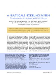
17.2 Multiscale Modeling 17.2.1 Lattice Dynamics Note that a crystalline material is distinguished from other states of matter by a periodic arrangement of the atoms, which can be represented as a collection of unit cells and a group of discrete and distinct atoms situated within each unit cell as depicted in Fig. 17.1. Consider a system consisting of Nl unit cells; each unit cell consisting of Na atoms with mass mα , [α = 1, 2, 3, . . . , Na ], positions Xkα in the reference configuration, xkα (t) in the current configuration at time t. Herein, the superscript kα refers to the α-th atom in the k-th unit cell. The displacements and velocities are ukα (t) = xkα (t) − Xkα and u˙kα ≡ dukα /dt. The initial configuration of each unit cell in a single crys talline material can be identified by its lattice coordinates k = (k1 , k2 , · · · , kd ) ∈ Z d , where d denotes the dimensions of space. So

=

+ Lattice

Figure 17.1

Basis

Atomistic view of crystal structure. See also Color Insert.


625

March 6, 2013

15:5


17-Shaofan-Li-c17


ath atom


X

Figure 17.2

ΔXka ka

k th unit cell

Xk

Position descriptions in the reference configuration.

the spatial initial position Xk of the k-th unit cell is obtained as d

Xk =

ka Ba

(17.1)

a=1

where Ba are the basis vectors spanning a simple d-dimensional Bravais lattice. The positions, shown in Fig. 17.2, in the reference configuration, displacements and velocities between atoms and the center of the unit cell are Xkα = Xk + �Xkα

(17.2)

ukα (t) = uk (t) + �ukα (t)

(17.3)

u˙kα (t) = u˙k (t) + �u˙kα (t)

(17.4)

where �Xkα , �ukα , and �u˙kα are the internal positions, internal displacements and internal velocities of the α-th atom in the k-th unit cell, respectively. The unit cell deformation uk (t) is homogenous, while the internal displacement �ukα (t) contributes to inhomogeneous deformation. It is assumed that the total potential energy V of the system can be additively computed as the sum of potential energies of each atom V =

V kα k

(17.5)

α

where the potential energy associated with the α-th atom in the k-th unit cell, V kα , is the sum of the energies due to any atomic interaction, such as pair-wise interaction of the atoms, three-body potentials or other many-body potentials, including the Tersoff and


March 6, 2013

15:5


17-Shaofan-Li-c17

Multiscale Modeling

the Stillinger–Weber potentials. V kα can be expressed in a general form 1 1 V2 (xkα , xlβ ) + V3 (xkα , xlβ , xmγ ) + · · · V kα = 2! l β 3! l,m β,γ


(17.6) with the understanding (k, α) = (l, β) = (m, γ ) = . . . . The particular form of the interatomic potential energy depends on the model of atomic interactions. In this work, we employ pair potential and the potential energy of atom kα is expressed as V kα =

1 2

V2 (xkα , xlβ ) ≡ l

β

1 2

V kα−lβ (xkα , xlβ ) l

(17.7)

β

Let the kinetic energy and the dissipative energy of this system be K =

1 2

mα (x˙kα )2 k

� D=

(17.8)

α

� 1 2

k

α

mα (x˙kα )2

(17.9) τ where D is ordinarily known as Rayleigh’s dissipation function and represents the rate at which mechanical energy is converted to heat during a viscous process; τ is a characteristic damping time [38]. We start from the generalized Lagrange equation for holonomic non-conservative systems, in which non-potential forces exist: d dt

∂L ∂x˙

−

∂L ∂D + = φ(x, x˙, t) ∂x ∂x˙

(17.10)

where L (x, x˙, t) = K –V is the Lagrangian and φ(x, x˙, t) is the generalized non-potential forces. Substituting Eqs. (17.7–17.9) into Eq. (17.10) and assuming that the forces on any atom are additive, after complicate but straightforward derivations, we have the governing equation of any atom kα in the system with damping mα u¨kα + c α u˙kα = fkα + φkα

(17.11)

kα−lβ ; where u˙kα = x˙kα ; u¨kα = x¨kα ; c α ≡ mα /τ ; fkα = l

βf kα

kα−lβ φ is the external force acting on the kα atom; f is the atomic


627

March 6, 2013

15:5


17-Shaofan-Li-c17



force acting on the kαatom due to the lβ atom, which is the negative derivative of the potential energy V kα−lβ (xkα , xlβ ) with respect to the atom’s current position vector xkα ∂ V kα−lβ (xkα , xlβ ) fkα−lβ = − (17.12) ∂xkα and here we also assume that the potential�energies depend only on � the relative interatomic distance d kα−lβ = �xkα − xlβ �, so

∂ V kα−lβ (d kα−lβ ) ∂d kα−lβ

∂d kα−lβ ∂xkα kα−lβ kα−lβ kα (d ) x − xlβ ∂V =− = −flβ−kα kα−lβ ∂d d kα−lβ

fkα−lβ = −

(17.13)

17.2.2 Kinematic Constraints For the purpose of large-scale simulation of collaborative material behavior, to reduce the computational time while maintaining the accuracy of the computational scheme, we seek an approximation solution to Eq. (17.11). Following the works by Knap and Ortiz [20] and by Eidel and Stukowski [39], the reduction of degrees of freedom is accomplished by virtue of kinematic constrains, may also be named as shape functions in finite element (FE) method or Cauchy–Born rule. Some judiciously selected unit cells, called FE nodes, retain their independent degrees of freedom and feature the deformation response of the system. Z is the set of all unit cells; Z N is the set of all FE nodes; Z N ⊆ Z . The nodal displacements together with shape functions are employed to determine a displacement field, in other words, all other unit cells are forced to follow the motion of the nodes — this is what we called “kinematic constraint,” which is the practice in every FE analysis. The most general requirements to the discretization are first, to reduce the number of FE nodes, and second, to ensure high density of FE nodes up to fully atomic resolution in critical regions, where defects nucleate and evolve, like dislocation cores, crack tips. When coarse mesh is used, the majority of the degrees of freedom can be eliminated, hence, the computational cost can be reduced while accompanying the decrease of the accuracy of the results associated with the computational scheme adopted. When the finest mesh is used, any lattice site is a finite element node, and the model becomes identical


March 6, 2013

15:5


17-Shaofan-Li-c17


Multiscale Modeling

to a full-blown MD model, the standard model manifesting the discrepancies or accuracies of others models by comparisons. The compromise is a trade-off between efficiency and accuracy. The density of FE nodes is controlled by a criterion that measures how strong the deformation varies spatially. Kinematic constraint means that the displacement ukα is approx imated by � I (k)UαI

ukα =

(17.14)

I

where � I (k) is I -th shape function evaluated at the k-th unit cell; UαI is the displacements of the α atom at the I -th node of the element in which the k-th unit cell resides. The finite element shape functions exhibit the properties � I (k) = 1

(17.15)

I

�I ( j ) = δI j

∀ j ∈ ZN

(17.16)

According to Eq. (17.15), shape functions follow the rule of “partition of unity” over Z , which ensures the exact representation of constant fields. Since the virtual work done by the atomic force fkα on the kα-th atom is � � � I (k)δUαI

fkα · δukα = fkα ·

{� I (k)fkα } · δUαI ; (17.17)

=

I

I

therefore, the nodal force contributed by the atomic force can be obtained as FαI = fkα � I (k)

(17.18)

Following the standard procedure of principle of virtual work, we have the weak form of Eq. (17.11) as follows: mα u¨ kα δukα + k

α

cα u˙ kα δukα = k

α

+

fkα−lβ δukα α

k

l

β

φ δu kα

k

kα

(17.19)

α

In light of fkα−lβ = −flβ−kα , we rewrite Eq. (17.19) as k α = 12 k

mα u¨kα δukα + α

l

β

{f

k kα−lβ


α

kα c α u˙kα δu

− flβ−kα }δukα + k

α

φkα δukα

(17.20)

629

March 6, 2013

15:5


17-Shaofan-Li-c17


which can also be written as


k α = 12 k

mα u¨ kα δukα +

c α u˙ kα δukα

k

α

l

β

α kα

fkα−lβ {δu

− δulβ } + k

α

φkα δukα

(17.21)

α By utilization of δukα = I � I (k)δU I , the governing equations α for nodal displacements U I can be expressed: � � � �

M IJα

U¨αJ +

C IJα

J

U˙αJ = FαI + �αI

(17.22)

J

where M IJα =

mα � J (k)� I (k) = M JIα

(17.23)

c α � J (k)� I (k) = C JIα

(17.24)

k

C IJα = k

FαI =

1 2

fkα−lβ � I (k) − k

l

β

�αI =

1 2

fkβ−lα � I (l) (17.25) k

l

φkα � I (k)

β

(17.26)

k

The existence of superscript α in Eq. (17.22) implies that the atomic information is naturally built in this coarse-grained molecular dynamics (CG-MD) method and the internal deformation is allowed in each node to represent an atomistic multi-element system, thereby eliminating the mismatch of phonon descriptions in atomic and continuum regions. Hence CG-MD is inherently suitable for the study of polarizations and phase transformations in multi element crystals at continuum level which cannot be reproduced by the classical continuum field theory. It is also noteworthy that, in Eqs. (17.25) and (17.26), full-blown nonlocality, nonlinearity and atom-based constitutive relation are automatically rooted in the force calculation, indicating that we propose a fully nonlocal CG-MD formulation which can appreciate the full benefit of the molecular dynamics while maintaining the computational efficiency due to the employing of the kinematic constraints. It is possible to envision that the use of this modeling methodology in support of diverse


March 6, 2013

15:5


17-Shaofan-Li-c17

Multiscale Modeling

Continuum region

Atomic region

Φ kJ w p f ka – lb

Φ kI w p f ka – lb

J

I

wq f h – ma

P

G


h

k

w p f ka – lb

yq

l

Φ kK w p f ka – lb

Φ kL w p f ka – lb

wq f ma – h

w p f lb – ka

m

H

L

Q

K

yp

a node; which is a unit cell

a unit cell

Figure 17.3 Schematic picture of coarse-grained model with force distributions. See also Color Insert.

applications, ranging from the simple full MD simulations to the simulations of MEMS and NEMS devices. For the sake of practical implementation, the consistent mass matrix is commonly replaced by a lumped mass matrix resulting in computational convenience. Here, we utilize the “row-sum” lumping technique enjoying a great popularity in dealing with the mass matrix, then Eq. (17.22) can be rewritten as � � ˜ Iα U¨αI + M

C IJα

U˙αJ = FαI + �αI

(17.27)

J

The complexity that arises in investigating the dynamics behav ior of material system is vastly due to the fact that many deformation phenomena involve multiple length and time scales, for example, from dislocation nucleation at atomic scale to the formation of multiple slip bands at submicron scale, to the observable effect of plastic deformation at the macro scale. Our attempts to unveil the distinctive physical phenomena across multiple scales in a single framework require modeling the material system in two distinctive regions: continuum region (Nl unit cells; each unit cell has Na atoms) with finite element meshes and atomic region (N atoms),


631

March 6, 2013

15:5


17-Shaofan-Li-c17



as shown in Fig. 17.3 (here a 2D picture is shown for the purpose of illustration). We can extend CG-MD method to a concurrent multiscale modeling method which addresses multiple length and time scale by encompassing different methods in a single analysis. Then the governing equations of this composite system can be expressed as Continuum region [α = 1, 2, 3, . . . , Na ] � � ˜ Iα U¨ αI + M

C IαJ

U˙ αJ = FαI + �αI

(17.28)

J

where the interatomic force FαI is a little bit different from Eq.

(17.25) because we should include the interaction with atoms in the

atomic region:

FαI =

1 2 k

fkα−lβ � I (k) − β

l

1 2

fkβ−lα � I (l) k

l

β

N

+

fkα−η � I (k) k

(17.29)

η=1

˜ Iα , the damping matrix C IJα and The diagonalized mass matrix M α the external force � I are the same as in Eqs. (17.23), (17.24), and (17.26). Atomic region [η = 1, 2, 3, . . . , N ] mη u¨η (t) = Fη (t) + �η (t)

(17.30)

η

where � (t) is the external force acting on the η-th atom, and the interatomic force acting on the η-th atom Fη (t) is Fη =

fη−kα + k

α

fη−ξ

(17.31)

ξ

17.2.3 Summation Rules on Force Calculations All summations in Eqs. (17.23)–(17.26), (17.29), and (17.31) are normally carried out by numerical quadrature. In Fig. 9.3, it is seen that around each node (an open circle), say the k-th node, there is a cluster (a shaded area), named ψk . From now on, force calculation is no longer performed for all unit cells in the entire system but for all clusters. A representative l unit cell (a black solid square) is the


March 6, 2013

15:5


17-Shaofan-Li-c17


Multiscale Modeling

one within one of ψk = {l : |Xl − Xk | ≤ Rk }. Notice that there is no overlapping of clusters. Xl is the position of the l-th unit cell and R k is the radius of the cluster ψk centered at the k-th unit cell, which happens to be a FE node. We postulate that the cluster summation rule for Eq. (17.29) reads: 1 1 FαJ = fkα−lβ � J (k) − fkβ−lα � J (l) 2 k l β 2 k l β Nl

w

N

fkα−η � J (k) ≈

+ k η=1

1 i 2 i ∈Z

N

Nl

Na

f N

f j α−lβ � J ( j )

j ∈ψi l=1 β=1 wi

w

1 i − 2 i ∈Z

Na

j ∈ψi

N

f j α−η � J ( j )

� J (l) +

jβ−lα

j ∈ψi l=1 β=1

i ∈Z N η=1

(17.32) where wi (i ∈ Z N ), the weight of the i th cluster, is calculated under the requirement that the summation over all linear interpolation functions must be exact [20, 39]. When the clusters shrink to nodes, i.e., ψi = {i }∀ i ∈ Z N , it holds � I (i ) = δ I i , and the cluster summation rule boils down to a node-based summation rule w

FαJ =

1 i 2 i ∈Z wi

Nl

N

Na

w

δ J i fi α− lβ −

l=1 β=1

1 i 2 i ∈Z

Nl

N

Na

fi γ −lα � J (l)

l=1 γ =1

N

+

fi α−η δ J i

(17.33)

i ∈Z N η=1

In this case, the weighting factor wi is the number of unit cells Nl represented by i -th node, thus wi = j =1 �i ( j ) ∀i ∈ Z N . On the other extreme case, wi = 1∀ i ∈ Z N implies all pairs of interatomic forces are calculated. In all cases i ∈Z N j ∈ψi w j = Nl holds. Figure 9.3 shows the numerical procedures to calculate the interatomic force between any two atoms. The force between any two atoms in the atomic region is treated exactly the same way as in MD simulation. In the continuum region the force between any two atoms in different or same unit cells should be distributed to all the nodes of the elements, in which the two unit cells reside. For example, there is a unit cell l located in cluster ψ H with weighting factor w H and another generic unit cell k; {fkα−lβ , flβ−kα } represents


633

March 6, 2013

15:5




a pair of interatomic forces acting on the kα-th atom and the lβ th atom fkα−lβ = −flβ−kα ; through shape function �kI = � I (k), force w H �kI fkα−lβ is distributed to the α-th atom of node I ; similarly, w H �k J fkα−lβ , w H �kK fkα−lβ , and w H �kL fkα−lβ are distributed to the α-th atom of nodes J , K , and L ; in the same way, w H �l J flβ−kα , w H �l K flβ−kα w H �l G flβ−kα and w H �l H flβ−kα are distributed to the β th atom of nodes J , K , G , and H . Let {fmα−η , fη−mα } represent a pair of interatomic forces acting on the mα-th atom in the continuum region and the η-th atom in the atomic region.

17.3 Multiple Physics In the past decade, the fact that “small is different” has been estab lished for a wide variety of multiple physical phenomena, including electrical, thermal, magnetic, and mechanical behavior. However, our attempts to analyze and reconcile the discrepancies between simulation-based results and experimental ones in multiple physical materials are hindered by our lack of fundamental understanding of these materials’ intricate multiple physics background within a single theoretical or computational framework. It is our hope that after reading this section the thermal-mechanical-electromagnetic coupling will simulate extensive research, establishing an apex shared between many discipline promoting integration and collabo ration.

17.3.1 Non-Equilibrium Molecular Dynamics Simulation Classical molecular dynamics simulations are performed in the microcanonical ensemble, meaning that we control the volume, the number of atoms and the energy. It is unable to provide statistical characters to the physical problem that it simulates. To extrapolate statistical thermodynamics information from molecular dynamics simulations, the performance of equilibrium ensemble molecular dynamics are required at a fixed temperature or fixed pressure or specified chemical potentials. Several methods have been introduced to keep the temperature constant while using the microcanonical ensemble. Popular techniques to control tempera


17-Shaofan-Li-c17

March 6, 2013

15:5


17-Shaofan-Li-c17


Multiple Physics

´ ture include velocity rescaling [40–46], the Nose–Hoover thermostat ´ [47, 48], Nose–Hoover chains [49], and the Berendsen thermostat [50]. The central idea is to simulate in such a way that we obtain a canonical distribution. Here, we briefly introduce the essence of ´ Nose–Hoover equilibrium MD, which is the most popular scheme within molecular dynamics community. In order to control the temperature of a specific region through which the thermal effects are brought into picture, the atomistic ´ or molecular controlled system is regularized by a Nose–Hoover thermostat. The governing equation of the conventional Nosé– Hoover MD simulation takes the following form: mi xï (t) = fi (t) + φi (t) − mi χ (t)x˙i (t)

(17.34)

where xi (t) is the position of the i -th atom; mi is its mass; fi (t) is the interatomic force acting on the i -th atom; φi (t) is the external force acting on the i -th atom; x˙i (t) = dxi (t)/dt; xï (t) = d 2 xi (t)/dt2 ; and χ (t) is a friction coefficient that may be controlled by the following equation: � � dχ (t) 1 T = 2 −1 (17.35) dt τ Teqb where Teqb is the expected temperature; τ is a specified time constant (normally in the range between 0.5 ps and 2 ps; T is the temperature, which can be calculated as a space-averaged variable N

3N kB T =

¯ 2 mi (vi − v)

(17.36)

i =1

In Eq. (17.36), kB is the Boltzmann constant; N is the total number of atoms in the controlled region; for atoms that do not reside in the controlled region, χ (t) = 0; vi = x˙i ; v¯ is the mass weighted average velocity of the controlled region. The action of the thermostat, featuring the interaction between the controlled region and its surrounding environment, is evidently an artificial force endowed on the controlled region offering an av enue for temperature control. Whenever the (kinetic) temperature of the atoms in the whole system T is larger than Teqb , χ (t) will increase and eventually become positive. Accordingly, the friction acts as a dissipation agent which will reduce the temperature.


635

March 6, 2013

15:5


17-Shaofan-Li-c17



Since the opposite occurs whenever the temperature falls below ´ thermostat represented by −mi χ (t)x˙ i (t) acts Teqb , the Nose–Hoover as a stabilizing feedback, similar to the controller in the robotic system. The total artificial force F and the total artificial moment L due to the action of thermostat are calculated as N

mi vi ≡ −χ P

(17.37)

mi xi × vi ≡ −χ H

(17.38)

F ≡ −χ i =1 N

L ≡ −χ i =1

We may call P and H as artificial linear momentum and artificial angular momentum, respectively. However, from Eqs. (17.37) and (17.38), the procedure of thermostat fails to make the artificial momenta vanish. In general, the artificial momenta should be zero; otherwise, the heat exchange between the system and the environment will lead to rotations and translations of the whole system, contradicting the observable macroscopic physi cal phenomena. Failure to guarantee the vanishing of the ar tificial momenta due to the implementation of the thermostat ´ insinuates that the conventional Nose–Hoover thermostat may mistakenly bring the unphysical phenomenon into the theory or simulation, spoiling the dynamic characterization of the whole system. To overcome the unphysical phenomenon emanating from the ´ thermostat, we propose an upgraded Nose–Hoover thermostat for non-equilibrium processes. Let the evolution of the atoms in the region which has thermal contact with the heat reservoir be ruled by mi v˙ i (t) = fi (t) + φi (t) − mi χ (t)(vi + �vi − v¯)

(17.39)

where �vi (t) is called the thermostat’s auxiliary velocity to make sure that the artificial momenta of the thermostats vanish during the whole process. The dynamics of χ is still governed by Eq. (17.35). ´ To illustrate the procedure of the upgraded Nose–Hoover thermostat, we need to define the following quantities:


March 6, 2013

15:5


17-Shaofan-Li-c17

Multiple Physics

The position vector of the centroid of the temperature-controlled region consisting of N atoms N

N

mi xi

i =1 N

R≡

≡

(17.40)

M

mi


mi xi

i =1

i =1

The relative position vector of atom i ri ≡ xi − R

(17.41)

The average velocity of the controlled region N

mi vi

i =1 N

v¯ ≡

P M

≡ mi

(17.42)

i =1

The angular momentum relative to the centroid N

¯ = H

mi ri × vi ,

� � ¯� H¯ ≡ �H

(17.43)

i =1

The moment of inertia of the controlled region N

mi ri · ri

I ≡

(17.44)

i =1

Now we propose the following procedures: Step 1 v˜i ≡ vi − v¯ It is seen that N

N

P˜ ≡

mi v˜ i = i =1

N

˜ = H

i =1 N

P =0 M N

m (R + r ) × (v − v¯) =

m x × v˜ = i i

i =1

mi (vi − v¯) = P − M

i

i

i

i =1

i =1

Step 2 vî ≡ v˜i + �vi


mi ri × vi = 0

i

637

March 6, 2013

15:5


17-Shaofan-Li-c17


where ˜ /I �vi = ri × H Then the artificial linear momentum and the artificial angular momentum, P and H, based on vî are calculated as


N

N

mi vˆ i =

Pˆ ≡ i =1

N

mi (v˜i + �vi ) = P˜ + i =1

˜ /I = 0 mi ri × H i =1

N

N

mi xi × vî =

ˆ = H i =1

mi (R + ri ) × (v˜i + �vi ) i =1

N

˜ + =H

mi (R + ri ) × �vi i =1 N

˜ + =H

N

˜ /I = mi ri × ri × H i =1

˜ )ri /I = 0 mi (ri · H i =1

Step 3 Calculate ˆ /I �vi = ri × H and update vî as vî ← vî + �vi Step 4 ˆ , based on the updated vî are The artificial momenta, Pˆ and H calculated as N

Pˆ ≡

N

mi vˆ i = i =1

N

mi �vi = i =1

ˆ /I = 0 mi ri × H i =1

N

ˆ = H

mi xi × vî i =1

� � ˆ � /H¯ is less than a specified tolerance, Now we make a test. If �H go to Step 6; otherwise go to STEP 5. Step 5 ˆ /I �vi = ri × H


March 6, 2013

15:5


17-Shaofan-Li-c17

Multiple Physics

ˆ /I vî ← vî + �vi = vî + ri × H Go to Step 4


Step 6 Finally the upgraded Nos´ e–Hoover Thermostat is expressed as mi v˙ i = fi + φi − χ (t)mi vˆ i N

3N kB T =

mi (vi − v¯)2 i =1

17.3.2 Coarse-Grained Non-equilibrium Molecular Dynamics Simulation To improve the computational efficiency and to broaden the applica tions of non-equilibrium molecular dynamics (NEMD) simulation, it is necessary to develop a coarse-grained non-equilibrium molecular dynamics (CG-NEMD) simulation technique with direct simulations of non-equilibrium systems with spatial temperature gradients. Figure 17.4 is a conceptual illustration of the CG-NEMD algo rithm. In Fig. 17.4, the gray solid circle means a unit cell; the blue solid circle means a FE node; the area surrounded by the red line is named as nodal ensemble with node I , i.e., the Wigner–Seitz region of node I, which contains a large number of unit cells. In the proposed model, we assume that each nodal ensemble is viewed as

Figure 17.4 Coarse-grained finite element meshes and the nodal ensemble. See also Color Insert.


639

March 6, 2013

15:5


17-Shaofan-Li-c17



a thermal reservoir, of which a unique temperature is defined. Note that the nodal ensemble is defined by Wigner–Seitz region, which depends on the FE discretization. The essence of the proposed CG-NEMD algorithm is: the FE nodes’ motion is determined by the external mechanical and thermal loading; whereas the atom’s motion in each finite element is controlled by the corresponding FE nodes through the shape functions; each FE node’s temperature is calculated through the motion of atoms in the corresponding nodal ensemble. The comparison between the temperature of nodal ensemble and the desired temperature, a feedback to the controllable FE node, drives the system. Since at the coarse scale level the temperature distribution is not uniform and evolves with time, the FE nodal temperature changes from node to node and from time to time. Therefore, if one wants to control the temperature of a set of specified nodes, a distributed ´ Nose–Hoover thermostat network is necessary to ensure that each nodal ensemble reaches to a desired temperature. This is called ´ ´ a generalized Nose–Hoover thermostat. The conventional Nose– Hoover thermostat renders the MD system a canonical ensemble, while this proposed model offers a coarse-grained canonical ensemble, a generalized notion of canonical ensemble in non equilibrium simulation. ´ Following the idea of Nose–Hoover thermostat, a damping force, with possible positive and negative damping coefficient, is used as an external force in FE analysis for coarse-grained non-equilibrium process. Following Eq. (17.28), assuming the damping coefficient cα ´ vanishing, the upgraded Nose–Hoover thermostat is proposed at the coarse level for each FE node as ˜ Iα (VαI − V¯ I + �VαI ) ˜ Iα U¨αI = FαI + �αI − χ I M M

(17.45)

where VαI = U˙αI is the velocity of the α-th atom at node I ; �VαI is the auxiliary velocity to make sure that the action of the thermostat itself does not alter the linear and angular momenta of the I -th nodal ensemble; V¯ I is the mass-weighted average velocity of all the atoms associated with node I -th node; the governing equation of χ I


March 6, 2013

15:5


17-Shaofan-Li-c17

Multiple Physics

is given as 1 dχ I = 2 dt τ NI

Na


3N I Na kB TI =

TI −1 Teqb−I mα (vkα − V¯ I )2

(17.46)

k=1 α=1

α where vkα = I � I (k)V I is the velocity of the kα-th atom in the nodal ensemble; N I is the number of unit cells associated with node I -th node; Teqb−I is the desired temperature of the I -th node. Note that in a specific non-equilibrium problem, not all FE ´ nodal temperatures are controlled, so the upgraded Nose–Hoover thermostat is merely employed at the FE nodes of interest, of which the temperature are controlled. On the other hand, if one wants to control the temperature of a group of FE nodes, one can assemble the group of FE nodes as a single thermal reservoir.

17.3.3 Electromagnetic Effects Advances from the integration of theoretical, computational and experimental techniques over the past years have revealed that piezoelectric materials have great potential for a variety of ap plication ranging from energy harvesting, sensing, actuation, to artificial muscles. More recently, a plethora of attentions have concentrated on exploring the nature of the electromechanical coupling at nanoscale, lending insights into the design principles for novel engineering piezoelectric devices. For example, Wang and co workers presented remarkable works demonstrating how electrical energy can be harvested from bending the ZnO nanowires by using atomic force microscope [51]. The quantitative exploitations of nanoscale mechanisms from the materials science perspective have advanced our ability to identify many unprecedented physical notions such as creating piezoelectric effects from non-piezoelectric materials, giant piezoelectricity in inhomogeneously deformed nanostructures, and ferroelectric properties, etc. Polarization, from the continuum viewpoint, restricts to non centrosymmetric crystal systems, featuring that an applied uniform strain can induce an electric polarization and vice versa. However, from the atomistic perspective, the polarization, associated with


641

March 6, 2013

15:5


17-Shaofan-Li-c17



piezoelectric properties, is a function of charges and positions of atoms in a unit cell. At atomic level, the polarization P is defined as the dipole moment per unit volume e (17.47) P= Z n Rn �V n where Rn is the position vector of charge Z n , e is the unit of charge, �V is the volume containing all the atoms in question. Consequently, it is straightforward to show the polarization density P(xk , t) of a lattice point in the coarse-grained molecular dynamics model as P(xk , t) =

1 Vcell

Na

q α �xkα

(17.48)

α=1

where q α is the charge of the α-th atom, Vcell is the volume of the unit cell, �xkα is the current relative position of the kα-th atom with re spect to the centroid of unit cell k. Equation (17.48) can give us both the local and bulk values of the polarization of a finite size specimen. Similarly, we can formulate the voltage and electrical field induced by the motion of the charged particles, which characterize the basis of the electromechanical coupling physics to appreciate the full benefits of energy harvesting. The induced voltage and electrical field can be expressed as Nl

V ind (xk , t) =

Na

(xk − xl ) q α �xlα · � � �xk − xl �3 l=1, xl =xk α=1 Nl

Na

Eind (xk , t) =

q α �xlα

l=1, xl =xk α=1

�

(17.49)

I 3(xk − xl ) ⊗ (xk − xl ) × −� � � � �xk − xl �3 �xk − xl �5

� (17.50)

It is noticed that all the electrical quantities including po larization, voltage and electrical field are expressed in terms of atomic motions. The atomic motions can be obtained from the balance law of linear momentum with interatomic potentials, leading to positions, velocities and accelerations. The coarse-grained molecular dynamics model proposed in this chapter inherently


March 6, 2013

15:5


17-Shaofan-Li-c17


Summary

holds the ability for elucidating the mechanism of polarization at nanoscale and serves as a novel avenue to the fundamental understanding of the nanoscale electromechanical and nanoscale energy harvesting. The riveting scenario, the mechanical deformations trigger the evolution of the electrical quantities, has been extensively discussed in the above sections. On the other hand, since φkα is the force due to external fields, it can be the Lorentz force due to the external electromagnetic field, which will generate the mechanical and electrical responses. The Lorentz force is depicted as φkα = q α (E + vkα × B/c)

(17.51)

where q α is the charge of the α-th atom; c is the speed of light; E is the electric field; and B is the magnetic induction; vkα is the velocity of the kα-th atom. Therefore, by accounting for the external Lorentz force, induced electrical quantities, and non-equilibrium temperature effects, the coarse-grained molecular simulation model presented in the chapter offers a novel path to investigate the thermal-mechanical-electromagnetic coupling phenomena.

17.4 Summary Simulation-based engineering science has emerged as a powerful tool revolutionizing engineering and science in the 21st century. It plays a major role in multiscale material modeling and design. While serving as a corner stone of many novel applications in all engineering disciplines from the nanoscale to macroscale, multiscale modeling and simulation has been revolutionized in the past decade by the emergence of experimental and computational techniques to study the properties and behaviors of materials near atomic/molecular scales. A fundamental understanding of the structure-property relationships of materials from the atomic scale to continuum scale within the multiple physics picture offers a novel avenue to make a breakthrough in current materials design technology. However, it remains elusive as to how the structural organization affects the material properties such as mechanical, thermal, electrical, and other properties.


643

March 6, 2013

15:5




With this impetus, this chapter presents a novel coarse-grained molecular dynamics methodology for dynamics simulations with the coupling effects of thermal, mechanical, and electromagnetic fields, offering a viable and high-potential research avenue to unravel the mechanism of how the multiscale structures and the multiphysics interact in the following three ways: 1. Literature in multiscale material modeling and simulation has struggled to strike a reliable balance over years between the computational efficiency and the accuracy of results involved in systems. Here, the authors choose a cluster-based summa tion rule for atomic force calculations in the finite element formulations. By implementing the different discretization, the simulation model in question can be evolved from a nodal-based simulation, to a cluster-based simulation, all the way to a full blown molecular dynamics simulation. 2. Many complex materials consist of more than one kind of chemical elements, for example, PbTiO3 , which hinders lots of multiscale material modeling methods incapable of capturing some exciting physical phenomena such as polarization, phase transition. It should be emphasized that the concept of unit cell (for example, considering PbTiO3 as a unit cell with five independent atoms) has laid a unique foundation for the CG MD proposed in this chapter, which bestow our methodology its invaluable property to investigate the missing physical phenomena uncovered in many other methods. 3. Multiple length and multiple physics have emerged as an indis pensible process of designing novel materials and charactering complex material properties. Up until now, theories describing multiple length and multiple physics in a single framework ´ are still lacking. By accounting for the upgraded Nose–Hoover thermostat and Lorentz force, we put forth a novel way to appreciate the full benefit of coupling the thermal, mechanical and electromagnetic fields at nano/micro scale. No research, however, provides a perfect answer, with this work being no exception to the rule. Based on current assumptions employed in implementing CG-MD, more work remains to be done. Specifically, the coupling of electromagnetic is one-coupling, which


17-Shaofan-Li-c17

March 6, 2013

15:5


17-Shaofan-Li-c17

References


means the magnetic field has no effect on the electric fields. Thus, more theoretical work should be devoted to explore and complement the full spectrum of the multiphysics coupling. The authors hope that this study can catalyze further work in the multiscale modeling of multiple physics.

Acknowledgments The co-authors, Xianqiao Wang, James D. Lee, and Azim Eskandarian, greatly appreciate the support from the Federal Highway Adminis tration of the US Department of Transportation under the award No. DTFH61-10-H-00005. The authors would also like to thank Dr. Kunik Lee for his helpful and enlightening discussions.

References 1. Liu, W.K., E.G. Karpov, and H.S. Park, Nano mechanics and materials: theory, multiscale methods and applications. 2006, Chichester, England; Hoboken, NJ: John Wiley. xiii, 320 p. 2. Oden, J.T., Simulation-based engineering science: revolutionizing en gineering science through simulation. Report of the National Science Foundation Blue Ribbon Panel on Simulation-Based Engineering Sci ence, K.P. Chong, cognizant program director, 2006. 3. Prater, C.B., H.J. Butt, and P.K. Hansma, Atomic force microscopy. Nature, 1990. 345(6278): pp. 839–840. 4. Dao, M., C.T. Lim, and S. Suresh, Mechanics of the human red blood cell deformed by optical tweezers. J Mech Phys Solids, 2003. 51(11–12): pp. 2259–2280. 5. Astbury, W.T., and H.J. Woods, X-ray studies of the structure of hair, wool, and related fibres. II.–The molecular structure and elastic properties of hair keratin. Proc R Soc Lond B, 1934. 114(788): pp. 314–316. 6. Tai, K., F.J. Ulm, and C. Ortiz, Nanogranular origins of the strength of bone. Nano Lett, 2006. 6(11): pp. 2520–2525. 7. Espinosa, H.D., Y. Zhu, and N. Moldovan, Design and operation of a MEMS-based material testing system for nanomechanical characteriza tion. J Microelectromech Syst, 2007. 16(5): pp. 1219–1231.


645

March 6, 2013

15:5



8. Espinosa, H.D., et al., Merger of structure and material in nacre and bone - Perspectives on de novo biomimetic materials. Prog Mater Sci, 2009. 54(8): pp. 1059–1100.


9. Abraham, F.F., and J.Q. Broughton, Large-scale simulations of brittle and ductile failure in fcc crystals. Comput Mater Sci, 1998. 10(1–4): pp. 1–9. 10. Rudd, R.E., Concurrent multiscale simulation and coarse-grained mole cular dynamics. Abstr Pap Am Chem Soc, 2001. 221: pp. 208–216. 11. Belytschko, T., and S.P. Xiao, Coupling methods for continuum model with molecular model. Int J Multiscale Comput Eng, 2003. 1(1): pp. 115– 127. 12. Xiao, S.P., and T. Belytschko, A bridging domain method for coupling continua with molecular dynamics. Comput Methods Appl Mech Eng, 2004. 193(17–20): pp. 1645–1669. 13. Wagner, G.J., and W.K. Liu, Coupling of atomistic and continuum simulations using a bridging scale decomposition. J Comput Phys, 2003. 190(1): pp. 249-274. 14. Fish, J., et al., Concurrent AtC coupling based on a blend of the continuum stress and the atomistic force. Comput Methods Appl Mech Eng, 2007. 196(45–48): pp. 4548–4560. 15. Parks, M.L., P.B. Bochev, and R.B. Lehoucq, Connecting atomistic-to continuum coupling and domain decomposition. Multiscale Model Simul, 2008. 7(1): pp. 362–380. 16. Shen, S.P., and S.N. Atluri, Multiscale simulation based on the meshless local Petrov-Galerkin (MLPG) method. CMES-Comput Model Eng Sci, 2004. 5(3): pp. 235–255. 17. Ma, J., et al., Multiscale simulation using generalized interpolation material point (GIMP) method and molecular dynamics (MD). CMESComput Model Eng Sci, 2006. 14(2): pp. 101–117. 18. Raghavan, P., and S. Ghosh, Adaptive multiscale computational modeling of composite materials. CMES-Comput Model Eng Sci, 2004. 5: pp. 151– 170. 19. Tadmor, E.B., M. Ortiz, and R. Phillips, Quasicontinuum analysis of defects in solids. Philos Mag, 1996. 73(6): pp. 1529–1563. 20. Knap, J., and M. Ortiz, An analysis of the quasicontinuum method. J Mech Phys Solids, 2001. 49(9): pp. 1899–1923. 21. Kulkarni, Y., J. Knap, and M. Ortiz, A variational approach to coarse graining of equilibrium and non-equilibrium atomistic description at finite temperature. J Mech Phys Solids, 2008. 56(4): pp. 1417–1449.


17-Shaofan-Li-c17

March 6, 2013

15:5


17-Shaofan-Li-c17

References

22. Steinmann, P., A. Elizondo, and R. Sunyk, Studies of validity of the Cauchy–Born rule by direct comparison of continuum and atomistic modelling. Model Simul Mater Sci Eng, 2007. 15(1): pp. S271–S281.


23. Tadmor, E.B., et al., Mixed finite element and atomistic formulation for complex crystals. Phys Rev B, 1999. 59(1): pp. 235–245. 24. Chen, Y.P., Local stress and heat flux in atomistic systems involving three-body forces. J Chem Phys, 2006. 124(5): pp. 054113. 25. Chen, Y.P., Reformulation of microscopic balance equations for multiscale materials modeling. J Chem Phys, 2009. 130(13): pp. 134706. 26. Chen, Y.P., and J.D. Lee, Atomistic formulation of a multiscale theory for nano/micro physics. Philos Mag, 2005. 85: pp. 4095–4126. 27. Lee, J.D., X.Q. Wang, and Y.P. Chen, Multiscale material modeling and its application to a dynamic crack propagation problem. Theor Appl Fracture Mech, 2009. 51(1): pp. 33–40. 28. Lee, J.D., X.Q. Wang, and Y.P. Chen, Multiscale computation for nano/micromaterials. J Eng Mech-ASCE, 2009. 135(3): pp. 192–202. 29. Wang, X.Q., and J.D. Lee, Wave propagating across atomic-continuum interface. Philos Mag Lett, 2011. 91(5): pp. 375–386. 30. Wang, X.Q., J.D. Lee, and Q. Deng, Modeling and simulation of wave propagation based on atomistic field theory. J Appl Mech-Trans ASME, 2011. 78: pp. 021012. 31. Xiong, L.M., and Y.P. Chen, Effects of dopants on the mechanical properties of nanocrystalline silicon carbide thin film. CMES-Comput Model Eng Sci, 2008. 24(2–3): pp. 203–213. 32. Xiong, L.M., and Y.P. Chen, Coarse-grained simulations of single-crystal silicon. Model Simul Mater Sci Eng, 2009. 17(3): pp. 035002. 33. Xiong, L.M., and Y.P. Chen, Multiscale modeling and simulation of single crystal MgO through an atomistic field theory. Int J Solids Struct 2009. 46(6): pp. 1448–1455. 34. Xiong, L.M., Y.P. Chen, and J.D. Lee, Atomistic simulation of mechanical properties of diamond and silicon carbide by a field theory. Model Simul Mater Sci Eng, 2007. 15(5): pp. 535–551. 35. Xiong, L.M., Y.P. Chen, and J.D. Lee, A continuum theory for modeling the dynamics of crystalline materials. J Nanosci Nanotechnol, 2009. 9(2): pp. 1242–1245. 36. Wang, X.Q., and J.D. Lee, Effects of electric fields on nanocrack propagation. Int J Fracture, 2011. 169: pp. 27–38.


647

March 6, 2013

15:5



37. Wang, X.Q., and J.D. Lee, Atomistic simulation of MgO nanowires subject to electromagnetic wave. Model Simul Mater Sci Eng, 2010. 18(8): pp. 085010.


38. Goldstein, H., C.P. Poole, and J.L. Safko, Classical Mechanics. 3rd ed. 2002, San Francisco: Addison Wesley. xviii, 638 p. 39. Eidel, B., and A. Stukowski, A variational formulation of the quasicontin uum method based on energy sampling in clusters. J Mech Phys Solids, 2009. 57(1): pp. 87–108. 40. Baranyai, A., and aacute, Heat flow studies for large temperature gradients by molecular dynamics simulation. Phys Rev E , 1996. 54(6): pp. 6911. 41. Muller-Plathe, F., A simple nonequilibrium molecular dynamics method for calculating the thermal conductivity. J Chem Phys, 1997. 106(14): pp. 6082–6086. 42. Lepri, S., R. Livi, and A. Politi, Thermal conduction in classical low dimensional lattices. Phys Rep, 2003. 377(1): pp. 1–80. 43. Poulikakos, D., S. Arcidiacono, and S. Maruyama, Molecular dynamics simulation in nanoscale heat transfer: A review. Microscale Thermophys Eng, 2003. 7(3): pp. 181–206. 44. Castejon, H.J., Nonequilibrium molecular dynamics calculation of the thermal conductivity of solid materials. J Phys Chem B, 2002. 107(3): pp. 826–828. 45. Tokumasu, T., and K. Kamijo, Molecular dynamics study for the thermal conductivity of diatomic liquid. Superlattices Microstruct, 2004. 35(3– 6): pp. 217–225. 46. Chantrenne, P., and J. Barrat, Finite size effects in determination of thermal conductivities: comparing molecular dynamics with simple models. ASME J Heat Transfer, 2004. 126: pp. 577–585. 47. Hoover, W.G., Canonical dynamics - equilibrium phase-space distribu tions. Phys Rev A, 1985. 31(3): pp. 1695–1697. 48. Hoover, W.G., and C.G. Hoover, Nonequilibrium molecular dynamics. Condens Matter Phys, 2005. 8(2(42)): pp. 247–260. ´ 49. Martyna, G., M. Klein, and M. Tuckerman, Nose–Hoover chains: the canonical ensemble via continuous dynamics. J Chem Phys, 1992. 97: pp. 2635–2645. 50. Berendsen, H.J.C., et al., Molecular-dynamics with coupling to an external bath. J Chem Phys, 1984. 81(8): pp. 3684–3690. 51. Wang, Z.L., and J.H. Song, Piezoelectric nanogenerators based on zinc oxide nanowire arrays. Science, 2006. 312(5771): pp. 242–246.


17-Shaofan-Li-c17

A Multiscale Modeling of Multiple Physics

A Multiscale Modeling of Multiple Physics

Suggest Documents

A Multiscale Modeling of Multiple Physics

A physics based multiscale modeling of cavitating flows - Dynaflow, Inc.

MULTISCALE MODELING AND SIMULATION OF

Multiscale neuronal modeling - arXiv

a multiscale modeling system - Colorado State University

Modeling Multiscale Landscape Structure Within A

Multiphysics & Multiscale Modeling, Data-Model

Hierarchical Stochastic Modeling for Multiscale

Multiscale agent-based cancer modeling

Hydromechanical Modeling Framework for Multiscale

Multiscale modeling of interaction of alane clusters

Multiscale geometric modeling of macromolecules I: Cartesian ...

Multiscale, Multiphysics Numerical Modeling of ...

multiscale modeling: thermal conductivity of graphene

Multiscale modeling and simulation of deformation in

Computationally Efficient, Fully Coupled Multiscale Modeling of ...

Review of Hierarchical Multiscale Modeling to

Statistical Multiscale Modeling of Smart Polymer

A review of predictive nonlinear theories for multiscale modeling of ...

Multiscale finite element modeling of nonlinear magnetoquasistatic ...

Multiscale Modeling of Turbulence, Radiation and ... - CiteSeerX

Multiscale modeling of multiferroic nanocomposites - Hal

Morphological and Multiscale Modeling of Stochastic ...

Multiscale Modeling of the Atomic Layer