A Nested Recursive Approach to MAP. Estimation based on Gauss-Markov Random Fields. â. J. Kaufhold. W. C. Karl. D. A. CastaËnon. BME Dept., Boston ...
A Nested Recursive Approach to MAP Estimation based on Gauss-Markov Random Fields
∗
J. Kaufhold
W. C. Karl
BME Dept., Boston University
ECE and BME Depts., Boston University
ECE Dept., Boston University
44 Cummington St, Boston MA
8 St Mary’s Street, Boston MA
8 St Mary’s Street, Boston MA
Abstract
D. A. Casta˜ non
time problems, such as arise in physical oceanography, space-time inverse scattering problems, visual field reconstruction and functional MRI (fMRI). A popular approach to regularizing such problems in a statistical context is via a Gauss-Markov Random Field (GMRF) prior model in a Maximum A Posteriori (MAP) estimation framework. While such approaches provide good reconstructions, the difficulty in their direct application to large spatial or spacetime problems is that their exact solution leads to impractically large and complex optimization problems due to high dimensionality. This limits the practical applicability and power of such GMRF-based formulations, particularly in real or near-real time applications. In this work we combine existing results on the recursive structure of GMRFs with reduced order model-based recursive filtering techniques to present a rational basis for approximate, model-based, recursive approaches to efficiently solve such problems.
Many large multidimensional space-time signal processing and data inversion applications (e.g. deconvolution) require some form of regularization to extract meaningful information. A popular approach to regularizing such problems in a statistical context is via a Gauss-Markov Random Field (GMRF) prior model in a Maximum A Posteriori (MAP) estimation framework. While providing good reconstructions, the high dimensionality of these problems can lead to prohibitive computational constraints which limit their practical applicability, particularly in real or near-real time applications. It has recently been shown that GMRF models posess a particular recursive structure. Conversely, complementary work in suboptimal filtering has been based on reduced order GMRF modeling. In this work, we combine these two results to present a suboptimal filter design which repeatedly takes advantage of this recursive GMRF structure to subdivide a large problem into a series of smaller, more Problem Statement tractable problems. In this way we present a method 2 for approximate, model-based, recursive solution to such high dimensional problems based on their inher- For simplicity, we will consider MAP estimation problems of the following form: ent recursive structure.
1
y = x + w, w ∼ N (0, R) x ∼ N (0, M )
Introduction
(1) (2)
where M corresponds to the covariance of a GMRF and R is the diagonal covariance of the observation noise, w. In particular, M −1 has a sparse banded structure reflecting the nearest neighbor interactions of the lexicographically ordered data [1]. The problem in (1) and (2) is representative of many estimation problems. For example, M is often chosen to capture a “smoothness prior” in which case M −1 ≈ DT D, where D is a derivative operator. The challenge posed by the applications we are considering is due to size and dimensionallity. For example, consider the space-time problem posed by enhancing a 3D fMRI data set. In this problem, we would need
Many large multidimensional space-time signal processing and data inversion applications require a method of regularization to extract meaningful information. These applications include large static spatial deconvolution problems, such as noise supression in 3D diffusion-weighted (vector-valued) magnetic resonance imagery (MRI) and mine detection in EM ground sensor array data, as well as space∗ This work was supported by a Whitaker Foundation Graduate Research Fellowship, the National Institutes of Health under Grant NINDS 1 R01 NS34189, by the Air Force Office of Scientific Research under Grant F49620-96-1-0028, and by the Army Research Office under Grant ARO DAAG55-97-1-0013.
1
to estimate over 109 elements (e.g. typical dimensions are 256 columns × 256 rows × 60 slices × 60 time points). Direct solution or inversion of corresponding normal equations is currently prohibitive if not impossible.
3
The blocks of G are related to the blocks of U as follows: G11 is the Cholesky factor of U11 . Gij = G−1 ii Uij for all off-diagonal blocks where i = j − 1, and Gjj is the Cholesky factor of Ujj − GTij Gij for all other diagonal blocks. Equations (3) and (4) can be derived from equation (1) and the Cholesky factor of M −1 in equation (5). First, defining equation (3) entails decomposing the diagonal covariance, R, and the observation vector, y, of equation (1) into subelements indexed to be compatible with the partitioning the equation (4). Now equation (4) is defined using the Cholesky factor T in equation (5). In particular, Q−1 n−i+1 = Gii Gii and T −1 An−i+1 = (Gii Gii ) Gij where j = i+1. This fact allows us to recast (1) and (2) as an equivalent dynamic estimation problem of the form given in equations (3) and (4). Note that this equivalence is exact, with no approximations. Conceptually, this dynamic model, obtained via Cholesky factorization, enables the optimal processing of the field with efficient techniques such as Kalman filter-based smoothing (e.g. Rauch, Tung, Striebel; Mayne-Fraser) algorithms. While this approach indeed transforms the original large problem into a sequence of smaller problems and while providing storage advantages, the overall amount of computation is still the same as that obtained if we exploited the banded MRF structure from the outset in the solution of the original complete normal equations. As we have argued, for the large practical problems we are considering, this amount of computation is still too large. Thus, to reduce the computational burden, some form of suboptimal approach is necessary. We discuss next a particular suboptimal approach to recursive filtering based on reduced order GMRF modeling of the estimation error field [1] which is particularly well-matched to our proposed solution.
Dynamic Reformulation
It is known that the inverse of the covariance matrix of a GMRF, M −1 in equation (2), termed the “potential matrix” in [3] and more commonly known as the “information matrix” [4], is sparse and banded with a particular structure. Recently, it was shown that the information matrix, M −1 of a GMRF possesses a certain highly interesting recursive structure [3]. Specifically, it was shown that the structure of the information matrix can be exploited to define an equivalent implicit autoregressive model on the subelements of the field of the form: yk xk+1
= xk + wk , wk ∼ N (0, Rk ) = Ak xk + vk , vk ∼ N (0, Qk )
(3) (4)
where the subelements xk and yk now define a “slice” (e.g. the rows or columns of an image) of the original field, and Rk and Qk are diagonal covariance matrices with compatible partitions. For appropriate choices of Rk , Ak , and Qk , It can be shown that that equations (3) and (4) yield the same overall covariance structure as the GMRF defined by M in the original problem. This equivalent dynamic model is derived through a Cholesky factorization of the corresponding information matrix, M −1 . To understand this, suppose we have a symmetric positive definite block tridiagonal matrix, M −1 = U of the following form: U11 U12 T U12 U22 U23 T U23 U33 U = .. . U
4
(n−1)n
GMRF-based Kalman Filter
In [1], an efficient suboptimal approach to Kalman filtering for large problems, such as in (3) and (4), is where U is composed of block tridiagonal subblocks, presented. In this development, a suboptimal variant Uii on the block diagonal and diagonal subblocks, of the information form of the Kalman Filter for (3) Uii+1 on the upper block off diagonal. Then we can and (4), consisting of the following prediction and uniquely decompose it as M −1 = U = GT G where G update steps is implemented: is the Cholesky factor of U and is of the form: PREDICTION STEP G11 G12 ∆ G22 G23 ˆ D = diag(ATk Q−1 (6) k Ak + Lk ) G 33 G= . (5) ∆ ˆ .. Ω = (ATk Q−1 (7) k Ak + Lk ) − D . G(n−1)n −1 −1 −1 Kk+1 = D − D ΩD . . . (8) Gnn T U(n−1)n
Unn
2
¯ k+1 L x ¯k+1 z¯k+1
−1 T −1 = Q−1 k − Qk Ak Kk+1 Ak Qk = Ak x ˆk ¯ k+1 x¯k+1 = L
(9) this way, we nest the recursive solution to the over(10) all high-dimensional problem, casting it as a series of progressively lower dimensional problems. This is the (11) original contribution of this work.
UPDATE STEP ˆ k+1 L zˆk+1 ˆ ˆk+1 Lk+1 x
¯ k+1 + R−1 = L k+1 = z¯k+1 + = zˆk+1
−1 Rk+1 yk+1
6
(12) (13)
6.1
(14)
Nested Solution
The main computational bottleneck in the approximate implementation of (6)-(14) can be traced to solving the implicit equation (14) for the updated state x ˆk+1 . In [1], (14) was solved iteratively by Gauss Seidel Successive Over Relaxation (SOR), exˆ k+1 . Note, however, ploiting the sparse structure of L that (14) can be viewed as another static spatial estimation problem, which is of the following form: yk+1 x ˆk+1
Incomplete Cholesky
While conceptually, a Cholesky factorization of M −1 in (2) provides the dynamics necessary to define an equivalent recursive smoothing problem, performing such a factorization is computationally prohibitive. The computational cost of computing an exact Cholesky factor of the block tridiagonal matrices we are considering following the definition given in Section 3 is O(nn3b ) where n is the number of blocks on the block diagonal, and nb is the dimension of each block. For instance, for the fMRI example discussed previously, n may correspond to 60 time points, and nb would be the number of voxels in each volume. In addition to the prohibitive computational cost of computing the Cholesky factor, fill-in occurs between the diagonal and off diagonal bands, destroying the structure of the problem so carefully preserved for efficiency in the suboptimal Kalman filter design in (6) through (14). Thus, in keeping with the reduced order GMRF modeling philosophy, we instead find an incomplete Cholesky factor, Ginc [2], such that ¯ In particular, the incomplete Cholesky GTinc Ginc ≈ L. factorization we use maintains the structure of the nearest-neighbor approximation scheme set up in the information form Kalman filtering equations. A range of incomplete Cholesky factorization algorithms appear in the computational linear algebra literature for preconditioning sparse linear systems. A problem with most incomplete Cholesky factorization algorithms is that their computational cost, although smaller than O(nn3b ), is not linear in the block size. For the problem sizes we are considering, we seek an incomplete Cholesky factorization with computational cost linear in the block size. The prohibitive computation in this process described in Section 3 can be traced to the inverse required for computing every off-diagonal block of the factor; this inverse is also the operation which leads to fill-in. For diagonally dominant diagonal blocks, Gii , this inverse may be well-approximated by the inverse of each block’s diagonal, which has computational cost O(nnb ) rather than O(nn3b ). This diagonal approximation to the inverse also imposes the overall sparsity pattern of the U matrix onto its factor, G. For applications we have examined, this approxima-
where, in the filtering equations above, as applied to (3) and (4), Kk+1 is a series expansion to ˆ −1 , L ¯ k+1 is the predicted informa(ATk Q−1 k Ak + Lk ) ˆ k+1 is the tion matrix, x¯k+1 is the predicted state, L updated information matrix, and xˆk+1 is the updated state as described in [1]. The suboptimal filter structure of [1] is based on the idea of imposing a reduced order GMRF-type model of the er¯ k+1 , the ror field, as reflected in the structure of L predicted information matrix in (9). In particular, ¯ k+1 is constrained to have a sparse, banded MRF L structure with the number of bands reflecting an imposed reduced-order GMRF neighborhood. Notice ¯ k+1 , is mainthat such a structure, once imposed on L ˆ k+1 . tained throughout (10)-(14) and imparted to L ˆ and L ¯ are conIn summary, at each iteration, L strained to have an MRF-like structure.
5
Approximations
= x ˆk+1 + vˆk+1 , vˆk+1 ∼ N (0, Rk+1 )(15) ¯ −1 ) ∼ N (0, L (16) k+1
¯ −1 again corresponds to where the prior model, L k+1 a covariance of a GMRF. This is true precisely because of the GMRF approximation imposed in (9). It is not true in the exact Kalman filtering equations ¯ k+1 is full in general. The problem in (15) where L and (16) is of the same form as the overall problem stated in equations (1) and (2). Therefore, we can apply the same technique we applied to solve the original problem, by performing a Cholesky factor of ¯ to again repose this subproblem as a dynamic estiL mation problem amenable to Kalman smoothing. In 3
1
tion is usually reasonable.
0.9
6.2
10
Dynamic and Observation Equations
0.8
9 8
0.7
7 0.6
6 Although the exact dynamic reformulation of the 5 0.5 GMRF MAP estimation problem in equations (1) 4 0.4 3 and (2) is given in Section 3, and the reformulation 2 0.3 is analogous for the incomplete Cholesky factor we 1 10 compute, certain operations in the reformulation de0.2 8 10 8 stroy the structure of the subproblems. In particu6 0.1 6 4 4 lar, the inverse in the definition of each Ak destroys 2 0 2 its GMRF structure, making it full in general. Because Q−1 k is constructed from the multiplication of Figure 1: Original Volume two nondiagonal matrices, it is no longer diagonal in general. As has been the modeling philosophy to alleviate similar issues in the rest of this paper, to main2 10 tain the required sparsity patterns for Q−1 and A , k k 1.5 9 we make sparse approximations to each. For Q−1 k , we 8 1 retain only its diagonal elements. For Ak , we make 7 6 the same two-term series expansion approximation 0.5 5 we make to Kk+1 in equation (8) of the Kalman fil4 0 3 ter, which again, is a rational approximation to the 2 −0.5 inverse which preserves the sparsity pattern of the un1 10 derlying GMRF model. However, even this approxi−1 8 10 mation to Ak is not completely adequate for the filter 8 6 −1.5 6 4 structure as it is presented in equations (6) through 4 2 2 ¯ k+1 will grow in (14). Specifically, the bandwidth of L ¯ equation (9). To remedy this issue, the Lk+1 matrix is Figure 2: Observed Volume truncated at every step through the filter, preserving its structure to reflect the original GMRF structure other pixels. In Figure 4, we show an example of our of the overall problem. nested recursive filtering method applied to processing the observed volume shown in Figure 2 given the 7 Examples normal equations corresponding to the GMRF model discussed above. We have implemented our nested recursive approach 0.9 to MAP estimation of Markov Random Fields on a test volume. The small example problem is an edge0.8 preserving smoothing operation. Three simultaneous 10 9 0.7 cross-sections of the underlying volume, a sphere of 8 ones on a background of zeros, are shown in a slice 7 0.6 display format in Figure 1. This underlying volume 6 5 0.5 is the state, x, we are trying to estimate in equa4 tions (1) and (2). This sphere is observed in white 3 0.4 2 Gaussian additive noise with diagonal covariance, or 1 0.3 r ∼ (0, R = 1/µI) in equation (1). The observation 10 8 10 is y = x + r, shown in Figure (2). The prior model 0.2 8 6 6 for the volume in equation (2) is a 3D GMRF prior 4 4 2 0.1 2 where M −1 is a discrete approximation to the gradient operator weighted by a function of the given Figure 3: Given Edge Locations edge process shown in Figure (3), such that the 3D GMRF prior has a large covariance at the pixels indicated by the edges, and a small covariance at all
4
9 1
10
We have combined a recursive interpretation of GMRF’s with an approximate information form Kalman filter based precisely on reduced order GMRF spatial models to develop a nested and efficient recursive approach to solution of GMRF regularized spatial estimation problems. In particular, we exploit the specific structure of the overall problem to reduce a large optimization problem into a series of dynamic equations amenable to solution by Kalman filtering techniques. We choose a specific information form Kalman filtering technique which allows us to exploit the sparse banded structure of the information matrix to make rational approximations to the prediction and update step. These approximations preserve the sparse banded GMRF structure of the original problem. Preserving this structure allows us to reformulate subproblems arising in the information form Kalman filter as a series of yet smaller dynamic equations. This nested recursive structure of the overall problem is elegant and also serves to make the solution more efficient. For higher dimensional problems, preliminary calculations suggest that this method will save more computation than traditional techniques for solving spatial estimation problems.
9 8 7
0.5
6 5 4 0
3 2 1 10
−0.5
8
10 8
6 6
4
4 2
2
Figure 4: Restored Volume (by nested recursion)
8
Conclusion
Discussion
In the edge-preserving smoothing example above, we illustrate 3 concepts. Most importantly, it demonstrates Kalman filtering as a means for volumetric data processing. Specifically, it illustrates the idea of splitting the GMRF neighborhood structure in 3D into an equivalent neighborhood structure in 2D along with a prior term which depends on the previous slice of data. This splitting is powerful, and can be used for multidimensional data where the state dimension may be much larger. Secondly, for such References an approach, the storage space for the sparse matri[1] T. M. Chin, W. C. Karl and A. S. Willsky. ces required to define the dynamic and observation Sequential Filtering for Multi-Frame Visual Reequations in the Kalman filtering grows linearly with construction. IEEE Trans. Sig. Proc., Spethe number of pixels in the volume. Finally, the comcial Issue on Multidimensional Signal Processing, putation is O(n) rather than O(n3 ), where n is the 28(3):311–333, Sept 1992. total number of elements in the field. for computing simultaneously the approximate MAP estimate [2] G. H. Golub and C. F. Van Loan. Matrix Comof the state as well as the approximate MAP estimaputations. Johns Hopkins Press, 1989. tion error. These are the primary motivations for the [3] J. Moura and N. Balram. Recursive Structure of suboptimal nested recursive filtering approach. Noncausal Gauss-Markov Random Fields. IEEE Trans. on Information Theory., 38(2):334–354, The specific performance of our method depends March 1992. on a host of factors, including the degree of diagonal dominance of the information matrices, and the order of the GMRF being processed. These factors are [4] P. S. Maybeck. Stochastic models, estimation and control. Academic Press, New York, 1979. consequences of the overall parameterization of the GMRF. Thus, the parameterization of the GMRF impacts the approximation error of the proposed nested recursive method. Specifically, for GMRFs enforcing strong regularization (i.e. for a large local correlation strength and large neighborhood sizes), approximation error will be larger. The relationship between smoothing in the GMRF definition and approximation error is of practical importance and is a focus of current investigation. 5