A networkbased framework for identifying ... - Wiley Online Library

PUBLICATIONS Water Resources Research RESEARCH ARTICLE 10.1002/2013WR014227 Key Points: Propose a connectivity-based conceptual framework of environmental response Present unit sedimentological responses for mud, sand, and gravel of a basin Resonant frequency of sediment supply leads to amplification of response

Correspondence to: E. Foufoula-Georgiou, efi@umn.edu

Citation: Czuba, J. A., and E. Foufoula-Georgiou (2014), A network-based framework for identifying potential synchronizations and amplifications of sediment delivery in river basins, Water Resour. Res., 50, 3826–3851, doi:10.1002/ 2013WR014227. Received 4 JUNE 2013 Accepted 22 APR 2014 Accepted article online 25 APR 2014 Published online 14 MAY 2014

A network-based framework for identifying potential synchronizations and amplifications of sediment delivery in river basins Jonathan A. Czuba1 and Efi Foufoula-Georgiou1 1

Department of Civil Engineering, St. Anthony Falls Laboratory, National Center for Earth-Surface Dynamics, University of Minnesota, Minneapolis, Minnesota, USA

Abstract Long-term prediction of environmental response to natural and anthropogenic disturbances in a basin becomes highly uncertain using physically based distributed models, particularly when transport time scales range from tens to thousands of years, such as for sediment. Yet, such predictions are needed as changes in one part of a basin now might adversely affect other parts of the basin in years to come. In this paper, we propose a simplified network-based predictive framework of sedimentological response in a basin, which incorporates network topology, channel characteristics, and transport-process dynamics to perform a nonlinear process-based scaling of the river-network width function to a time-response function. We develop the process-scaling formulation for transport of mud, sand, and gravel, using simplifying assumptions including neglecting long-term storage, and apply the methodology to the Minnesota River Basin. We identify a robust bimodal distribution of the sedimentological response for sand of the basin which we attribute to specific source areas, and identify a resonant frequency of sediment supply where the disturbance of one area followed by the disturbance of another area after a certain period of time, may result in amplification of the effects of sediment inputs which would be otherwise difficult to predict. We perform a sensitivity analysis to test the robustness of the proposed formulation to model parameter uncertainty and use observations of suspended sediment at several stations in the basin to diagnose the model. The proposed framework has identified an important vulnerability of the Minnesota River Basin to spatial and temporal structuring of sediment delivery.

1. Introduction For long-term prediction of the environmental response of a basin to natural and anthropogenic disturbances, physically based distributed models are of limited use as they need many input parameters which are hard to specify and predictions become increasingly uncertain as the prediction horizon increases. For example, the transport time scale for mud (silt and clay) can be of the order of hours to days (storm-event response), while for sand and gravel can be of the order of tens to thousands of years, depending on climate and basin characteristics. When predicting such long-term response, the specific magnitude of the predicted flux might not be very accurate but the timing of the maximum flux, and also the identification of areas of the basin contributing to that maximum flux are important for long-term planning and for assessing how human-changes on a naturally evolving landscape might inadvertently affect downstream changes in many years to come. Landscapes contain networks of dynamically connected paths (fluvial, hillslope, subsurface, etc.) that play an important role in structuring environmental fluxes and the overall basin response to a given input. An environmental response, defined as the time distribution of a quantity of interest (streamflow, sediment, nutrients, etc.) at the outlet of a basin due to a spatially distributed input, is structured by the network through time delays and transformations imposed by the physics of the environmental process operating on that network. Simplified approaches that take advantage of network topology, channel characteristics, and transport-process dynamics offer the possibility to identify hot spots or vulnerable areas/times of disturbance that can lead to synchronization and downstream amplification of the response. Inspired by the extensive linear systems theory approach to the hydrologic response [Sherman, 1932; Nash, 1957; Dooge, 1973; Kirkby, 1976; Rodriguez-Iturbe and Valdes, 1979; Gupta et al., 1980; Troutman and Karlinger, 1985; Gupta et al., 1986; Mesa and Mifflin, 1986; Gupta and Mesa, 1988; Maidment et al., 1996; Muzik,

CZUBA AND FOUFOULA-GEORGIOU

C 2014. American Geophysical Union. All Rights Reserved. V

3826

Water Resources Research

10.1002/2013WR014227

1996; Rinaldo et al., 2006a, 2006b; Botter et al., 2010] and its extension to the sedimentological response for mud at the storm-event time scale [Johnson, 1943; Williams, 1978; Kumar and Rastogi, 1987; Sharma et al., 1992; Raghuwanshi et al., 1994; Gracia-Sanchez, 1996; Lee and Singh, 1999; Kalin et al., 2004a, 2004b; Singh et al., 2008; Bhunya et al., 2010; Lee and Yang, 2010], we propose here a conceptual framework for computing the ‘‘sedimentological response function’’ of a basin focusing specifically on the transport of mud, sand, and gravel. The sedimentological response function is defined as the time distribution of the sediment quantity delivered to the outlet of a basin in response to an instantaneous unit input of sediment uniformly distributed over the basin. This response function is computed by performing a nonlinear process-based scaling of the network width function (the probability distribution of distances to the outlet) into a time response function. The framework incorporates not only the network topology but also (via process-based scaling) specific attributes of the three-dimensional structure of the landscape, stream morphology, and hydrodynamics that contribute to sediment production and transport, such as slope, depth, and width of the river at any location, shear stress of the bed, relevant magnitude/frequency of flow, etc. Using scaling functions (such as hydraulic geometry), the proposed framework can be considerably simplified and reduced down to a few parameters that can convert the network width function to a process-scaled response function. In this paper, we present the proposed framework for transport of mud, sand, and gravel and demonstrate it in a specific high sediment production regime in the Minnesota River Basin. This basin was selected as a prototype because excessive sediment impairs river water quality and biotic functioning, and the management of current and future actions on the landscape requires unraveling the temporal and spatial effects of these actions, as well as understanding how the environment continues to respond to past actions and disturbances.

2. Conceptual Framework of Environmental Response The proposed connectivity-based conceptual framework of environmental response relies on performing a physically based scaling of the distances (link lengths) along the network by characteristic velocities of the flux transported on the network to obtain the ‘‘environmental response function’’ for the flux of interest. The environmental response function provides significant insight into the ‘‘workings of the system’’ (in terms of both its structural components and dynamics) and provides a building block for computing the flux at the outlet of the basin in response to any temporally variable input in the basin, under of course, the proportionality and superposition assumptions of linear system theory. The theoretical basis of the proposed framework rests on the link between Lagrangian and Eulerian transport formalisms by which one can establish the relation between the evolution in time and space of the trajectories of an ensemble of particles injected over a set of points at an initial time and transported over all possible trajectories in the network, to the first passage (or travel time) distribution at a fixed control section, here at the outlet of the basin [e.g., Rodriguez-Iturbe and Rinaldo, 1997]. Let the river network be defined by a set of hierarchically connected links i, where a link is defined as the segment of the network between a source and a junction (a source link), two successive junctions, or a junction and the basin outlet. Junctions are the points at which two links join, sources are the points farthest upstream in the network, and the outlet is the point farthest downstream in the network. Each link i is assigned a geomorphic fluvial state nf ;i which may include geomorphologic and hydraulic attributes of the link, i.e., nf ;i ‘i ; ai ; Ai ; Si ; Qw;i ; Hi ; Bi ; ::: , where the geomorphologic attributes may include the link length ‘i 2 [L], directly contributing area ai [L ], upstream drainage area Ai [L2], and link slope Si, and the hydraulic attributes may include the streamflow Qw;i [L3 T21], cross-section average depth Hi [L], average width Bi [L], etc. (Figure 1a). While not indicated explicitly, attributes of the geomorphic state nf ;i may also be a function of time to capture possible time-varying properties of the system. Let now ci denote the pathway (set of links) that a particle initiating at link i will follow along the river network to reach the outlet. The properties of this pathway are defined by the hierarchical (directed) collection of the geomorphic fluvial states of the links composing ci, i.e., fni ; :::; nX g from the geomorphic state ni through the network to the outlet (i.e., ni ! ::: ! nX ). It is noted that, in general, a landscape can be seen as a set of connected paths, which in addition to fluvial paths might include hillslope, subsurface, floodplain, pond/wetland, pipe, etc., paths which can also be incorporated in the above framework if their properties are known. In what follows we restrict ourselves to fluvial paths only.



3827


10.1002/2013WR014227

b)

a) Fraction of links

W (x) 3

ξ f ,i

1

Fraction of links

Geomorphic fluvial state of link i :

(l , a , A , S , Q i

3

Distance to the outlet, L

2

ξ f ,i

2

1

i

i

i

c)

W p (t )

1 2

w,i , H i , Bi ,...)

3

Transport time to the outlet, T

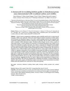
Figure 1. Conceptual framework of environmental response. (a) Illustration of a river basin with fluvial channel network. The highlighted segment of the network is a link i corresponding to geomorphic fluvial state nf ;i with associated attributes. Areas of the basin, such as 1, 2, and 3, sitting at a certain distance from the outlet contribute to (b) a specific structure of the width function W(x). (c) The contribution of these areas to the outlet may be redistributed in the process-scaled width function Wp ðtÞ based on the characteristics of the process of interest. The resulting environmental response function is a complex transformation of the original width function that depends on the river network topology and the attributes of the geomorphic fluvial states nf ;i for all i links.

A particle introduced into link i has a pathway distance Li [L] from that point to the outlet given by X Li 5 ‘j ;

(1)

j2ci

which is the sum of link lengths along pathway ci. The width function (WF) W(x) is defined as the number of links in the network (typically normalized by the total number of links) which are found at a discretized pathway distance x [L] from the outlet measured along the network (Figure 1b). Thus, in the limit of a large number of pathways, the WF is the probability distribution of pathway distances to the outlet of the basin. The directed network of link lengths ‘i [L] may be transformed to a directed network of travel times tp;i [T] based on a process operating on the network, say through a process-specific velocity up;i [L T21] of the transported environmental flux. The travel time tp;i is the time it takes a particle to move through (or the time during which a particle is in) geomorphic state ni and is given by tp;i 5

‘i : up;i

(2)

Note that tp;i must include both the time when the particle is actually moving and the time when it is not being transported, i.e., it stays in storage within link i. When long-term storage is present, then up;i represents a virtual velocity whose physical meaning has to be interpreted with caution. Here as detailed in section 3, long-term storage effects are ignored and only short-term storage (due to the intermittency of flood events capable of transporting sediment) is incorporated via an intermittency factor formalism (explained in more detail in Appendix B). Considering this length-to-time conversion, a particle introduced into link i has a pathway travel time Tp;i [T] to the outlet given by X Tp;i 5 tp;j ; (3) j2ci

which is the sum of travel times along pathway ci. Thus, when such transport dynamics are introduced on the river network, each pathway distance to the outlet is scaled to a travel time to the outlet. This allows one to compute the probability that a particle found at the outlet at time t [T] was in position x (and thus



3828


10.1002/2013WR014227

within an upstream link at distance x from the outlet) at time t 5 0. This distribution produces a processscaled width function (PSWF) Wp ðtÞ defined as the number of links in the network (normalized by the total number of links) that contribute to the outlet at time t (Figure 1c). This PSWF is also the probability distribution of pathway travel times of particles (introduced instantaneously and uniformly in all links in the network) to the outlet of the basin, and as such relates to the geomorphologic instantaneous unit response function (GIURF) of the basin. It is understood that the contributions of different areas of the basin to the WF may be considerably redistributed in the PSWF based on the characteristics of the process of interest (Figure 1); e.g., particles injected at two points which are at the same distance to the outlet might arrive at the outlet at significantly different times depending on the transport properties of their pathways (slopes, channel hydraulic properties, bed friction, etc.). Obviously, if the process-specific velocity up is constant for all links, the PSWF (normalized by the maximum process-specific pathway travel time Tp;max [T]) and the WF (normalized by the maximum pathway distance Lmax [L]) coincide. In section 3, the PSWF (or GIURF) is formulated for mud, sand, and gravel transport in a river network.

3. Formulation of the Sedimentological Response Function Sediment in large and small quantities is intermittently and spatially nonuniformly supplied to river networks [Benda and Dunne, 1997a, 1997b; Reid et al., 2007a] across a broad range of sizes that include clay ( sc;i , where sc;i 50:0495 for the Wong and Parker [2006] gravel-transport formula. The proposed formulation for gravel response only exists if the transport s;i 5



3836


10.1002/2013WR014227

threshold is exceeded everywhere in the basin (otherwise contributions from the basin can never be transported to the outlet). Therefore, the flow is capable of transporting gravel when, and the GIUS for gravel for the Minnesota River Basin only exists if,

Si >

sc;i Ri Di 2bHA Ai aHA

(36)

for the Q2. Considering the potential transport of sediment with a grain size of Di 5 0.01 m (8i; and the other parameters specified based on those given for the sand response function), the transport threshold is not exceeded everywhere in the basin for this formulation, and therefore, the gravel response function does not exist at the outlet of the basin at the Q2. This suggests that this size gravel is not transported out of the Minnesota River Basin at or below the Q2. For this reason, we do not go into further details about the gravel response and leave further investigations that consider spatially variable grain size, abrasion, and variable flow above the Q2, for a future study. However, mapping where the river system is capable of transporting gravel ðs;i 2sc;i > 0Þ would provide insight into potential transport and deposition areas of the network. While this map is not shown, the areas where the river system is capable of transporting gravel are those with the steepest slopes (Figure 3) in the knickzones of tributaries entering the main stem Minnesota River and in the northwestern part of the basin. Gravel supplied to channels capable of transporting this material will eventually be transported downstream (and abrade or break down into smaller particles) until it reaches a channel that is not capable of transporting this material. These downstream channels are potential deposition reaches for gravel as any gravel supplied to it would accumulate at this location. Additionally, channels capable of transporting gravel are those with the greatest capacity for erosion and these channels may indicate potential sediment sources where the river is capable of recruiting bank material into the channel.

5. GIUS of the Minnesota River Basin The proposed formulation of the GIUS describes how sediment with grain size Di instantaneously released and uniformly distributed over the basin would propagate (below transport capacity) through the river system to the basin outlet. We repeat that the present formulation only considers storage (time delays) for sediment on the bed or on bars that are readily mobilized by the next capable flow. Long-term storage of sediment due to floodplain deposition or meander migration over a bar that is re-entrained when the river sweeps back across the floodplain is not considered at present. Thus the proposed GIUS provides a lower bound on the fastest time scale for sediment to transport from different parts of the basin to the outlet. This is in contrast to the prodigious research on sediment pulses in rivers, where an emplaced pulse of sediment exceeds transport capacity and largely disperses in place [Lisle et al., 1997, 2001; Cui et al., 2003a, 2003b; Cui and Parker, 2005; Lisle, 2008; Sklar et al., 2009]. This section includes a description of the GIUS of the Minnesota River Basin, an evaluation of its robustness to model parameter uncertainty, and a diagnostics/validation analysis of the GIUS for sand using suspended-sediment data. 5.1. Description of the GIUS The pathway distance from each link to the outlet was grouped into seven bins to show the correspondence between the river network of the Minnesota River Basin and its WF (Figures 4a and 4b). The first two contributions to the WF (corresponding to areas at distances 0–100 and 101–200 km from the outlet in Figures 4a and 4b) are small which is reflected in the narrow width of the Minnesota River Basin near the outlet. The two peaks of the WF (corresponding to areas at distances 301–400 and 501–600 km from the outlet in Figures 4a and 4b) reflect the widest regions of the Minnesota River Basin and result from the structure of the network, where many links are within these distances from the outlet. The WF generated using 100 bins maintains the large-scale structure of the 7-bin WF but now conveys smaller-scale information on the network structure (Figure 4c). Three distinct regions of the WF emerge: a narrow region (between normalized distance 0 and 0.3), a central region (between normalized distance 0.3 and 0.7), and a distant region (between normalized distance 0.7 and 1; Figure 4c). Each region reflects



3837

Water Resources Research 600

0.04

a)

0.1

0

Fraction of links

400

Number of links

Fraction of links

600 0.2

0.2

0.4 0.6 0.8 Normalized distance

b)

1

c) 80

0.03 60 0.02 40 0.01

200

0

600

Width Function

800 0.3

Distance to the outlet, km 200 400

0

0

0

0.04

Distance, km

Fraction of links

0 - 100 101 - 200 201 - 300 301 - 400 401 - 500 501 - 600 601 - 700

Number of links

Distance to the outlet, km 200 400

0

20

0

0.2

0

40

0.4 0.6 0.8 Normalized distance

0

Time to the outlet, hours 80 120 160

Mud (Streamflow) Response Function

0.03

1

d) 80 60

0.02 40 0.01

Number of links

0.4

10.1002/2013WR014227

20

Outlet 0

0.04

0

0

0.2

0.4 0.6 Normalized time

0.8

1

0

Time to the outlet, years 100 200 300

Sand Response Function

e)

30

60

120 Kilometers

60 0.02 40 0.01

0

Number of links

0

Fraction of links

80 0.03

20

0

0.2


0.8

1

0

Figure 4. Width function and process-scaled width functions of the Minnesota River Basin. (a) Width function within seven discretized distance bands of the Minnesota River Basin corresponding to the (b) map of distances from each link to the outlet. (c) Width function within 100 discretized distance bands showing more fine-scale detail. (d) Process-scaled width function or geomorphic instantaneous unit sedimentograph for mud (streamflow). Note the time scale is on the order of hours to days. (e) Process-scaled width function or geomorphic instantaneous unit sedimentograph for sand (0.4 mm). Note the time scale is on the order of tens to hundreds of years.

contributions from different areas of the Minnesota River Basin. The PSWF or GIUS can be thought of as a WF generated from a network of pathway travel times rather than from a network of pathway distances. In this way, scaling link lengths by a characteristic velocity transforms the pathway-distance network nonuniformly into a pathway travel time network. The GIUS for mud (streamflow; Figure 4d) is similar in shape to the WF because the characteristic velocity for mud transport (streamflow velocity) weakly increases with drainage area (to the 0.07 power; equation (31)). If the characteristic velocity for mud transport was a constant throughout the basin, then the GIUS would be a linearly scaled version of the width function. However, because the characteristic velocity increases downstream, the pathway travel time network is similar to the pathway-distance network except for proportionally longer upstream links and shorter downstream links. The nonlinear scaling increases the delay of contributions from upstream links and decreases the delay from downstream links compared to



3838


10.1002/2013WR014227

the WF. The scaling of the GIUS for mud spreads out the link contributions which slightly reduces the peaks of the GIUS for mud compared to the WF. The GIUS for sand (Figure 4e) is substantially different from the WF with peaks concentrated at a normalized distance of 0.3 and 0.7. Substituting the scaling relation for the channel slope, obtained from the 30 m DEM as Si 5ð0:30Þ A20:31 ; i

(37)

into equation (33), simplifies the characteristic velocity for sand transport as a constant times the drainage area to the 20.18 power, us;i 50:05 Ai20:18 :

(38)

Therefore, the characteristic velocity generally decreases downstream resulting in a pathway travel time network with proportionally shorter upstream links (decreased delay of contributions) and longer downstream links (increased delay of contributions) compared to the pathway-distance network. Contributions from upstream links more quickly enter downstream links, which concentrate the contributions from upstream links and increase the peaks of the GIUS for sand compared to the WF. The structure of the sand response truly arises from the network topology, channel slopes, and sandtransport formulation.

5.2. Robustness and Validation of the GIUS for Sand The timing of the GIUS for sand is highly sensitive to three parameters (Di, hi, and If ;s ) which appear as linear multipliers in equation (19) and therefore uniformly shift the timing of the overall response, without however affecting the shape of the response. The GIUS for sand has been computed using the D50 sand size of Di 5 0.4 mm from riverbed material within the Minnesota River Basin (Figure 4e) [U.S. Geological Survey, 2013]. If instead the sand has a different median size, e.g., Di 5 0.3 or 0.5 mm, the timing of the response function changes such that, rather than obtaining peaks at 90 and 265 years (Di 5 0.4 mm), the peaks would occur at 70 and 200 years (Di 5 0.3 mm) or 115 and 330 years (Di 5 0.5 mm). Thus, there is an uncertainty in the timing of the peaks of the GIUS due to uncertainty in the choice of Di, hi, and If ;s . The shape of the GIUS for sand is only affected through the exponents on the upstream drainage area Ai and slope Si (see equations (19) and (33)) that contribute to the transport time in a nonlinear way to rearrange contributions to the GIUS for sand (Figure 5). The exponent of the upstream drainage area was varied from 0 to 0.5 and the exponent of slope was varied from 0 to 5/2 (Figure 5). Note that the exponents of zero correspond to the width function (Figure 5m; A0S0), which for different parameters, resulting from the specific transport dynamics, stretches to become the sand response function (Figure 5g; A0.285S3/2). Increasing the exponent on the upstream drainage area tends to smooth out the contributions to the response, whereas increasing the exponent on slope tends to concentrate contributions into peaks. For most of the variations in the exponents of the sand response function, the two peaks in the GIUS remain, although shifted, suggesting that bimodality is a relatively robust property of the GIUS for sand for the Minnesota River Basin. As an attempt to validate the formulation of the GIUS for sand, the best estimate of the rate of total sand transport at the 2 year flow Q2 (observed; Appendix C, approximately 120% of the rate of measured suspended-sand transport at the Q2) was compared to the simulated rate of total sand transport at the Q2 (simulated; Figure 6) computed as

Qs;i 5

0:05 3=2 3=2 u2 H Bi Si : g1=2 R2i Di w;i i

(39)

A few measurements show good agreement between the simulated and observed rates of total sand transport; however, most simulated rates are an order of magnitude larger than the observed rates (Figure 6). When comparing the relative differences between the simulated and observed transport rates with the upstream drainage area (Figure 6b), the best agreement occurs at sites with large drainage areas and at a



3839

Water Resources Research S^ 0.08

0

10.1002/2013WR014227

1/2

3/2

b)

a)

5/2 d)

c)

A^

0.06

0.5

0.04 0.02 0 0.08 e)

f)

g)


0.06

h)

0.285

Fraction of links

0.04 0.02 0 0.08 i)

j)

k)

l)

0.06

0.1

0.04 0.02 0 0.08

m)

n)

Width Function

0.06

o)

p)

0

0.04 0.02 0

0

0.2

0.4

0.6

0.8

1 0

0.2

0.4

0.6

0.8

1 0

0.2

0.4

0.6

0.8

1 0

0.2

0.4

0.6

0.8

1

Normalized time

a)

100

1

lin

e

1

1:

10

lin

e

10

0

Relative difference between simulated and observed rates of total sand transport, (Qs,sim - Qs,obs) / Qs,obs

1,000

1:

Simulated rate of total sand transport, kg/s

Figure 5. Sensitivity of the shape of the sand response function (geomorphologic instantaneous unit sedimentograph, GIUS). The sand response function arises from a characteristic velocity scaling A0.285S3/2 (Figure 5g; see equation (33)) due to the exponents on upstream drainage area and slope that rearrange contributions to the GIUS for sand compared to the width function (Figure 5m; A0S0). The exponent of upstream drainage area was varied from 0 to 0.5 (increases vertically) and the exponent of slope was varied from 0 to 5/2 (increases horizontally). Note that for most of the variations in exponents around the sand response function (Figure 5m) the two peaks in the GIUS remain, although shifted, suggesting that this is a relatively robust property of the GIUS for sand for the Minnesota River Basin.

0 1 10 100 1,000 Best estimate of observed rate of total sand transport based on suspended-sediment measurements, kg/s

70 b) 60 50 40 30 20 10 0 -10 100

1,000

10,000

100,000

Upstream drainage area, km2

Figure 6. Comparison of the observed to simulated rates of total sand transport. (a) The best estimate of the rate of total sand transport at the Q2 (observed; see Appendix C, approximately 120% of the measured rate of suspended-sand transport at the Q2) was compared to the simulated rate of total sand transport at the Q2 (simulated; see equation (39)). (b) Relative difference between simulated and observed rates of total sand transport compared to upstream drainage area. Note that the simulated rate of total sand transport represents atcapacity transport, independent of sediment supply, whereas the observations take into account spatially variable sediment supply as well as transport-limited behavior in the system. Likely this comparison identifies supply-limited (large discrepancy) versus transport-limited (small discrepancy) parts of the basin.



3840


10.1002/2013WR014227

Combined Response D = 1.41 mm D = 0.71 mm D = 0.35 mm D = 0.18 mm D = 0.09 mm Combined Response D = 1.41 mm D = 0.71 mm 1

0.8

Fraction

D = 0.35 mm

D = 0.18 mm

Fraction of links

D = 0.09 mm

0.6

0.4

0.2

0.02

0 0.01

0.1

1

10

Sediment grain size, mm 0.01

0 0

200

400

600

800

1000

1200

Time to the outlet, years Figure 7. The geomorphologic instantaneous unit sedimentograph (GIUS) for the grain-size distribution of sand on the riverbed within the Minnesota River Basin (see inset for grain-size distribution). The GIUS for the sand distribution was generated for each individual size, scaled according to relative abundance in the grain-size distribution, and then added together across sizes to obtain the combined response. Individual size responses and the combined response are offset vertically for ease of comparison. Note that the combined response reflects the GIUS for the mode of the grain-size distribution.

few sites with small drainage areas. Note that the simulated Qs;i represents at-capacity transport whereas the observations take into account the actual sediment supply. It is possible that the large discrepancy between rates indicates that the transport formula or parameters used in the transport formula are not appropriate, but we suggest that this comparison may identify supply-limited versus transport-limited parts of the basin. Some upstream parts of the basin might be supply limited (simulated sand-transport capacity >> observed transport), and at downstream links, homogenization of spatial and temporal variability may take place leading to transport-limited conditions (simulated sand-transport capacity 5 observed transport), which might indicate a potential for storage as any sediment supplied above capacity would go into storage. Nonetheless, where sediment supply may not be a limiting factor, there is relatively good agreement (within an order of magnitude) between the simulated and observed rates of total sand transport.

6. Partitioning Contributions to the Sedimentological Response The GIUS is a system property and represents the response of the system to a spatially uniform input of sediment. Typically, the sediment input in such a large basin would vary spatially and temporally and this would require convolving partitioned and scaled versions of the GIUS to realize the observed sedimentological response at the outlet of the basin. We illustrate how the GIUS can be partitioned and scaled into a



3841


10.1002/2013WR014227

Fraction of links

A

b)

Mud (Streamflow) Response Function

a)

Blue Earth River Basin

Time to the outlet, hours 80 120 160

40

0.03

80 60

Basin A+B 0.02

40

Basin B 0.01

Outlet

0

20

0

0.04 0

0.2

0.4 0.6 0.8 Normalized time Time to the outlet, years 100 200 300

Fraction of links


B

1

0.03

30

60

0

c) 80

A+B

60

B 0.02

40 0.01

0

Number of links

0

Number of links

0.04

20

120 Kilometers 0

0

0.2


0.8

1

0

Figure 8. Partitioning contributions to the sedimentological response highlights critical sediment source areas. (a) The partition of the Blue Earth River Basin (B; red) and the rest of the basin (A; gray). (b) Sedimentological response for mud for the entire basin (A1B; black) and for the Blue Earth River Basin (B; red). (c) Sedimentological response for sand (0.4 mm) for the entire basin (A1B; black) and for the Blue Earth River Basin (B; red).

sedimentological response by considering a mixture of sediment and contributions from subbasins of the Minnesota River Basin. The GIUS is specified for a specific grain size, such as the D50 sediment size, but in reality a mixture of sediment sizes is transported concurrently by the river network. Considering the grain-size distribution of sand on the riverbed within the Minnesota River Basin (inset Figure 7; [U.S. Geological Survey, 2013]), a GIUS for sand can be generated for each individual size, scaled according to relative abundance in the grain-size distribution, and then added together across sizes to obtain the combined response (Figure 7). Under the assumption that individual grain-size fractions sort during transport such that the transport of each fraction can be simply treated individually as a response and added together to obtain the combined response (which may not be accurate due to hiding effects [Wilcock and Crowe, 2003]), the combined response reflects the GIUS for the mode of the grain-size distribution. The framework developed herein allows partitioning of the contributions to the GIUS based on any attributes of the geomorphic state, e.g., different subbasins which might have distinct features or sediment contributions. The Minnesota River Basin was partitioned here into two subbasins: the Blue Earth River Basin and the rest of the basin to disentangle the contribution of each to the GIUS at the outlet of the basin (Figure 8). During 2002–2006, the Blue Earth River Basin contributed over 50% of the sediment supply to the Minnesota River Basin despite the fact that it only accounts for roughly 20% of the total area [Wilcock, 2009]. Therefore, sediment contributions from the Blue Earth River Basin to the GIUS are expected to be larger than from other areas of the Minnesota River Basin. It is seen from Figure 8b that the partitioned contribution from the Blue Earth River Basin to the GIUS for mud corresponds to the central region of the response between normalized distance 0.3 and 0.7. The partitioned contribution from the Blue Earth River Basin to the GIUS for sand concentrates into the first peak at a normalized distance of 0.3 (Figure 8c). It is important to note that scaling of the network topology based on the sand-transport process has shifted the contribution of the Blue Earth River Basin from the central region of the WF to the first peak of the GIUS for sand. This highlights that nonlinear spatial stretching of the network topology based on the sediment-transport process rearranges contributions to the GIUS in unexpected ways compared to the contributions to the WF.



3842

Disturbance events

Water Resources Research a)

d1

d2

Disturbance events generating an instantaneous input of sand uniformly over the entire basin e)

t=0 100 Number of links

10.1002/2013WR014227

t = 175

years

Response for d1

b)

80 A

60

A+B+C

A

40 20 0

Number of links

100

Response for d2

c)

80 A+B+C

60

B

Outlet

C

40 20 0 180

d)

Combined Response for d1 and d2

Number of links

160 140 120

C A+C

100 80 60

0

40

30

60

120 Kilometers

20 0

0

100

200 300 400 Time to the outlet, years

500

Figure 9. Synchronization of sediment fluxes can lead to amplification of the response for the Minnesota River Basin. (a) Disturbance of the landscape leading to two instantaneous inputs of sand (0.4 mm; uniformly over the basin) at 0 years (disturbance 1 or d1) and 175 years (disturbance 2 or d2). (b) Sedimentological response corresponding to d1; entire basin response (dashed line; basins A1B1C in Figure 9e) and region corresponding to the second peak of the sand response (blue shaded area; basin A in Figure 9e). (c) Sedimentological response corresponding to d2; entire basin response (dotted line; basins A1B1C in Figure 9e) and Blue Earth River Basin (red shaded area; basin C in Figure 9e). (d) Superimposed response for sand (sum of Figures 9b and 9c) into an observed response (black line) resulting in amplification of the effects of the sediment inputs. Amplification can also occur if only the regions contributing to the peaks of the response (basin A in Figure 9b and basin C in Figure 9c) are disturbed and responses superimposed (purple shaded area; A1C). (e) Partition of the basin into three regions: the region corresponding to the first peak of the sand response (red; C, Blue Earth River Basin), second peak of the sand response (blue; A), and the rest of the basin (gray; B).

7. Amplification of the Sedimentological Response As demonstrated in the previous sections, the shape of the GIUS of a basin carries the signature not only of the river network topology but also of the specific hydraulic and stream morphologic characteristics of the channels. As a result, the peak contributions at the outlet of a basin arise from the superposition of inputs that arrive at the outlet from disparate, and even unconnected, parts of the basin. Given the long response times of sediment transport in rivers, which may be of the order of hundreds or thousands of years, one could envision changes occurring in parts of the basin at decadal or longer time scales and the associated response progressing downstream and superimposing on past responses in such a way that leads to unexpected amplifications. In this section, we demonstrate this idea using the Minnesota River Basin and its sedimentological response for sand. Suppose a landscape disturbance event occurs which delivers an instantaneous input of sand (0.4 mm) uniformly over the entire basin at a time t 5 0 years (d1; Figure 9a). Such an event may be extreme precipitation, which detaches sediment and the resulting overland flow entrains and delivers this sediment directly to the river network. This was likely a common mechanism during the late 19th century and early 20th



3843


10.1002/2013WR014227

century when agricultural practices largely disturbed the landscape and left the top soil exposed and vulnerable to erosion. Extreme precipitation may also lead to very high streamflow capable of eroding and recruiting bank material into the channel. This is likely the most common mechanism today for delivering sand to the river network as soil-conservation practices have greatly improved and underground tile drainage has expanded [Belmont et al., 2011]. The sedimentological response at the outlet of a basin for the disturbance event at t 5 0 years (d1) is the GIUS for sand for the Minnesota River Basin (dashed line; Figure 9b). It is seen that the structure of the GIUS exhibits two peaks which arise from the network topology, channel slopes, and sand-transport formulation. The two prominent peaks suggest that there is a resonant frequency of sediment supply that would lead to an amplification of the response. Given regularly occurring sediment-transporting flows/events, two peaks are manifested in the response at 90 and 265 years (Figure 9b). If another landscape disturbance event occurs 175 years after the first which delivers an instantaneous input of sand (0.4 mm) uniformly over the entire basin at a time t 5 175 years (d2; Figure 9a), the additional contribution to the sedimentological response will be similar to the first but shifted in time (Figure 9c). This assumes that disturbance events (or events that deliver sediment) are less frequent than those that transport the sediment through the river network [Lane et al., 2008]. The observed response at the outlet of the basin (Figure 9d) is the superposition of the individual responses (Figures 9b and 9c) leading to an amplified sedimentological response, with a greatly increased peak at 265 years and a relatively long duration of high contributions from 250 to 280 years after the initial disturbance (Figure 9d). Conceptually, this suggests a 175 year resonance time (resonant frequency with a period of 175 years) for sand (0.4 mm) for the Minnesota River Basin. While the GIUS conceptualizes the sedimentological response to a uniformly distributed disturbance and input to the river network, in reality these disturbances are more localized within the basin. Amplification of the sedimentological response can still occur if only specific source areas are disturbed instead of the entire landscape. For instance, if the first disturbance event (d1; Figure 9a) only disturbed a northwest region of the basin (A; Figure 9e) the sedimentological response would be only a portion (the second peak) of the GIUS (blue shaded area; Figure 9b). If the second disturbance event (d2; Figure 9a) only disturbed the Blue Earth River Basin (C; Figure 9e) the sedimentological response would be only the portion (the first peak) of the GIUS (red shaded area; Figure 9c). These seemingly isolated disturbances (in both space and time), would be ordered, delayed, and superimposed into an observed and unexpectedly amplified sedimentological response at the outlet of the basin (purple shaded area; Figure 9d). When amplification of the sedimentological response occurs, likely there is an interaction between the two peaks that is not simply the sum of the two peaks. If the increased sediment supply to a channel is below the transport capacity, then the supply is transported downstream without a change in channel characteristics (change in channel slope or width). However, if the increased sediment supply overwhelms the transport capacity, which is likely the case, then the channel will aggrade and the change in channel characteristics will act to filter and reduce the peak of the increased sediment supply. Detailed processbased, reach-scale, sediment-transport models are best suited to quantify the specifics of the reach-scale changes due to increased sediment supply. However, this conceptual framework complements detailed process-based approaches by illuminating how inputs of sediment to the river system are structured by the river network and delayed in time due to the sediment-transport process. The amplification of the sedimentological response could result in greater than expected aggradation of the bed of the river leading to disruption in ecosystem function, increased flood risk, and increased cost associated with remediation. Therefore, the proposed framework has identified an important vulnerability of the Minnesota River Basin to spatial and temporal changes in the basin and suggests that aggregated effects need to be seen within a whole-network framework and not in isolation.

8. Concluding Remarks In this paper, we presented a connectivity-based conceptual framework of environmental response, focusing on the sedimentological response for mud, sand, and gravel. The proposed framework relies on performing a nonlinear process-based scaling of the network geometry (link lengths) to convert the network width function into a time response function or process-scaled width function (PSWF) where the process of interest is sediment transport. The process-scaled width function for sediment is the geomorphologic



3844


10.1002/2013WR014227

instantaneous unit sedimentograph (GIUS) or the sedimentological response of a basin to an instantaneous unit volume of sediment uniformly entering all links of the network. The proposed framework was applied to the Minnesota River Basin to aid in understanding its long-term sedimentological response to spatially and temporally varying changes in the landscape. It was shown that the network topology and sediment-transport dynamics in the Minnesota River Basin combine to produce a double peaked response function for sand, suggesting that there exists a resonant frequency of sediment supply that could lead to an unexpected downstream amplification of sedimentological response. The two peaks of the sand response function can be attributed to specific areas of the basin, highlighting that the disturbance of one region followed by the disturbance of another region after a certain period of time, may result in an amplification of the effects of the sediment inputs that is otherwise difficult to predict with mechanistic short-time horizon models. The synchronization and amplification of sediment delivery in specific places of a basin may result in greater than expected aggradation of the riverbed triggering disruption in ecosystem functioning, and leading to increased flood risk and increased cost associated with remediation. Therefore, the proposed framework has identified an important vulnerability of the Minnesota River Basin to spatial and temporal structuring of sediment delivery, and can aid in understanding how climatic trends and current and future management decisions may be unexpectedly superimposed on this landscape as it undergoes intensive human management while it is still adjusting to past geologic disturbances.

Appendix A: Hydraulic Geometry Scaling Hydraulic geometry scaling was based on field measurements from 23 USGS streamflow-gaging stations in the Minnesota River Basin (see Figure 2 for gage locations) [U.S. Geological Survey, 2013]. A representative bankfull flow at each gage was determined from a frequency analysis of annual peak flows, where bankfull flow was chosen as the 2 year recurrence interval peak flow (Q2 or 2 year flow [L3 T21]) and determined as the daily streamflow that has a 50% chance of being exceeded in any year. Then the hydraulic characteristics (uw;i [L T21], Hi [L], and Bi [L]) at the Q2 at each gage were obtained by regressing the measured hydraulic characteristics made during USGS streamflow measurements against streamflow, and taking the values of the hydraulic characteristics at the Q2 (figures not shown). Downstream hydraulic geometry relations were developed by regressing the Q2 with each hydraulic characteristic obtained at each gage for all 23 gages in the basin (Figures A1a–A1c). The downstream hydraulic geometry relations for the Minnesota River Basin were obtained as: Bi 5ð5:34ÞQ0:48 2;i ;

(A1)

Hi 5ð0:321ÞQ0:42 2;i ;

(A2)

uw;i 5ð0:583ÞQ0:10 2;i ;

(A3)

and

3

where Q2;i is specified in m /s, Bi in m, Hi in m, and uw;i in m/s. Typical exponents for these relations are 0.50, 0.40, and 0.10 for the Bi Q2;i , Hi Q2;i , and uw;i Q2;i scaling relations, respectively [Leopold and Maddock, 1953; Park, 1977], which are in close agreement with those of the Minnesota River Basin. It is noted that the velocity hydraulic geometry relation has a low coefficient of determination (R2 5 0.12; Figure A1c), highlighting the spatial heterogeneity in this basin which calls for a spatially explicit analysis. Additionally, the Q2 was found to scale with upstream drainage area, Ai [L], (Figure A1d) as Q2;i 5ð1:4e25ÞA0:70 ; i

(A4)

where Ai is specified in m2. Typically, this exponent is 0.75 and varies from 0.65 to 0.80 for bankfull flow [Leopold et al., 1964], which is in close agreement with that of the Minnesota River Basin. Combining the hydraulic geometry relations of equations (A1–A3) with equation (A4) gives the scaling of hydraulic characteristics with upstream drainage area for the Minnesota River Basin as: Bi 5ð0:024ÞA0:34 ; i



(A5)

3845


10.1002/2013WR014227

a) Bi = 5.3 Q2,i0.48 R2 = 0.87

Bi, m

102

101 101 b)

H i, m

Hi = 0.32 Q2,i0.42 R2 = 0.84

100

c)

uw,i, m/s

uw,i = 0.58 Q2,i0.10 R2 = 0.12 100

10−1 101

Q2,i, m3/s

103

102 Q2,i, m3/s

103

d) Q2,i = 1.4e−5 Ai0.70 R2 = 0.75

102

101 108

109

1010

1011

Ai, m2 Figure A1. Hydraulic geometry scaling based on field measurements at 23 U.S. Geological Survey streamflow-gaging stations in the Minnesota River Basin (see Figure 2 for gage locations) of (a) channel width, (b) flow depth, and (c) streamflow velocity versus the 2 year recurrence interval peak flow (obtained from a frequency analysis of annual peak flows for each station). (d) Scaling of the 2 year recurrence interval peak flow versus drainage area.



3846


10.1002/2013WR014227

Hi 5ð0:0029ÞA0:29 ; i

(A6)

uw;i 5ð0:20ÞA0:07 ; i

(A7)

and

where Ai is specified in m2, Bi in m, Hi in m, and uw;i in m/s.

Appendix B: Intermittency Factor for Sand Transport The intermittency factor for sand transport for the Minnesota River Basin was calculated at USGS streamflow-gaging station 05325000, Minnesota River at Mankato, Minnesota (see Figure 2 for gage location) and assumed to apply to the entire basin. The approach for determining the intermittency factor (first introduced by Paola et al. [1992]) follows the approach outlined by Parker [2004]. The volumetric transport rate of sand per unit width at the Q2 (2 year (bankfull) flow), qs;b [L2 T21], was computed using equations ((8), (13), (10), and (11)). Then the daily streamflow record at the Mankato gage was used to compute nonparametrically the kth-percentile daily streamflow, qk [L2 T21], and its corresponding probability of occurrence, pk. From qk, the volumetric transport rate of sand per unit width in the kth percentile, qs;k [L2 T21], was then computed for all k percentiles using equations ((8), s [L2 (13), (10), and (11)). Next, the mean annual volumetric transport rate of sand per unit width, q 21 T ], was computed as s5 q

X

pk qs;k ;

(B1)

k

by summing the product pk qs;k over all k percentiles. Finally, the intermittency factor for sand transport, If ;s , was computed as If ;s 5

s q : qs;b

(B2)

For the Minnesota River at Mankato, the intermittency factor for sand was computed as If ;s 50:175. This is the fraction of time per year that continuous Q2 would yield the mean annual sand load.

Appendix C: Best Estimate of the Rate of Total Sand Transport Estimates of the rate of total sand transport were obtained from suspended-sediment measurements at 18 USGS streamflow-gaging stations in the Minnesota River Basin (see Figure 2 for gage locations) as follows. At each gage, suspended-sediment concentration and sand fraction, if not a full grain-size distribution, was measured along with streamflow at different instants of time and flows [U.S. Geological Survey, 2013]. Suspended-sediment concentration and sand fraction at the 2 year recurrence interval peak flow (Q2) was estimated from the measurements at each gage. For the majority of sites, approximately 30% of the measured suspended sediment was sand at the Q2. The rate of suspended-sand transport at the Q2 was computed by multiplying the suspended-sediment concentration by the sand fraction and the Q2 streamflow. The rate of total sand transport at the Q2 was then computed following the method of Shah-Fairbank et al. [2011] (and using the method of Guo and Julien [2004] to compute the Einstein integrals) from the rate of suspended-sand transport at the Q2, bed shear stress (estimated from Q2 and channel dimensions), suspended-sediment fall velocity (estimated using the equation of Ferguson and Church [2004] and measured D50 sand size in suspension, 0.15 mm [U.S. Geological Survey, 2013]), and D65 of bed material (from bed-material measurements at gages, 1 mm [U.S. Geological Survey, 2013]). In the end, this method generally estimated the rate of total sand transport at the Q2 equal to approximately 120% of the measured rate of suspended-sand transport at the Q2, and represents the best estimate of the observed rate of total sand transport (including both suspended and bed load transport) at the Q2 from suspended-sediment measurements at gages.



3847


10.1002/2013WR014227

Notation ai Ai Bi Cf ;i Di g Hi i If ;g If ;s j k ‘i La;i Li Lmax pk qg;i qg;i qk s q qs;b qs;i qs;k qs;i Qg;i Qs;i Qw;i Q2 Ri Si t tp;i tg;i 0 tg;i ts;i 0 ts;i tw;i Tp;i Tp;max Tg;i Ts;i Tw;i up;i ug;i us;i uw;i W(x) Wp ðtÞ Wg ðtÞ Ws ðtÞ Ww ðtÞ


directly contributing area to the ith link [L2]. drainage area upstream of the ith link [L2]. channel width of the ith link [L]. friction coefficient of the ith link. sediment grain size in the ith link [L]. acceleration due to gravity [L T22]. cross-section averaged flow depth of the ith link [L]. index denoting spatial location within the network. intermittency factor for gravel transport. intermittency factor for sand transport. connectivity index along pathway ci. index of a percentile. length of the ith link [L]. active layer thickness of the ith link [L]. pathway distance from geomorphic state ni to the outlet [L]. maximum pathway distance [L]. probability of occurrence of the kth-percentile daily streamflow. volumetric transport rate of gravel through the ith link [L2 T21]. dimensionless volumetric transport rate of gravel through the ith link. kth-percentile daily streamflow [L2 T21]. mean annual volumetric transport rate of sand per unit width [L2 T21]. volumetric transport rate of sand per unit width at the 2 year (bankfull) flow [L2 T21]. volumetric transport rate of sand through the ith link [L2 T21]. volumetric transport rate of sand per unit width in the kth percentile [L2 T21]. dimensionless volumetric transport rate of sand through the ith link. volumetric transport rate of gravel through the ith link [L3 T21]. volumetric transport rate of sand through the ith link [L3 T21]. streamflow or volumetric transport rate of water through the ith link [L3 T21]. 2 year recurrence interval peak flow [L3 T21]. submerged specific gravity of sediment in the ith link. slope of the ith link. arbitrary arrival time of a particle at the outlet of a basin [T]. process-specific transport time through the ith link [T]. travel time of gravel through the ith link [T]. travel time of gravel through the ith link during constant bankfull flow [T]. travel time of sand through the ith link [T]. travel time of sand through the ith link during constant bankfull flow [T]. travel time of mud (streamflow) through the ith link [T]. process-specific pathway travel time from the ith link to the outlet [T]. maximum process-specific pathway travel time [T]. pathway travel time of gravel from the ith link to the outlet [T]. pathway travel time of sand from the ith link to the outlet [T]. pathway travel time of mud (streamflow) from the ith link to the outlet [T]. process-specific velocity through the ith link [L T21]. characteristic velocity of gravel in the ith link [L T21]. characteristic velocity of sand in the ith link [L T21]. characteristic velocity of the flow in the ith link [L T21]. width function. process-scaled width function. process-scaled width function for gravel transport. process-scaled width function for sand transport. process-scaled width function for mud transport (streamflow).


3848

Water Resources Research x ag aHA auw A bg bHA buw A ci hi nf ;i ni q sb;i sc;i s;i X

Acknowledgments This research was funded by NSF grant EAR-1209402 under the Water Sustainability and Climate Program. The first author acknowledges the support of a UMN Civil Engineering departmental fellowship and the second author acknowledges the support of the Joseph T. and Rose S. Ling Endowed Professorship. We sincerely thank Jim Pizzuto (Univ. of Delaware), Peter Wilcock (Johns Hopkins Univ.), and an anonymous reviewer for their insightful comments which helped improve the presentation of our work. We also thank the Editor (Graham Sander) and Associate Editor (anonymous) for an efficient and constructive review process.


10.1002/2013WR014227

arbitrary pathway distance from the outlet measured along the network [L]. coefficient of the gravel-transport formula. coefficient of the Hi Ai scaling relation. coefficient of the uw;i Ai scaling relation. exponent of the gravel-transport formula. exponent of the Hi Ai scaling relation. exponent of the uw;i Ai scaling relation. connectivity of geomorphic state ni to the outlet. scale factor for determining the characteristic vertical length scale for sand transport. geomorphic fluvial state of the ith link. geomorphic state of the ith link. density of water [M L23]. bed shear stress in the ith link [M L21 T22]. critical dimensionless bed shear stress for the initiation of motion in the ith link. dimensionless bed shear stress in the ith link. index of the basin outlet.

References Belmont, P. (2011), Floodplain width adjustments in response to rapid base level fall and knickpoint migration, Geomorphology, 128, 92– 102, doi:10.1016/j.geomorph.2010.12.026. Belmont, P., et al. (2011), Large shift in source of fine sediment in the Upper Mississippi River, Environ. Sci. Technol., 45, 8804–8810, doi: 10.1021/es2019109. Benda, L., and T. Dunne (1997a), Stochastic forcing of sediment routing and storage in channel networks, Water Resour. Res., 33, 2865– 2880, doi:10.1029/97WR02387. Benda, L., and T. Dunne (1997b), Stochastic forcing of sediment supply to channel networks from landsliding and debris flow, Water Resour. Res., 33, 2849–2863, doi:10.1029/97WR02388. Bhunya, P. K., S. K. Jain, P. K. Singh, and S. K. Mishra (2010), A simple conceptual model of sediment yield, Water Resour. Manage., 24, 1697– 1716, doi:10.1007/s11269-009-9520-4. Botter, G., E. Bertuzzo, and A. Rinaldo (2010), Transport in the hydrologic response: Travel time distributions, soil moisture dynamics, and the old water paradox, Water Resour. Res., 46, W03514, doi:10.1029/2009WR008371. Clayton, L., and S. R. Moran (1982), Chronology of late Wisconsinan glaciation in middle North America, Quat. Sci. Rev., 1, 55–82. Cui, Y., and G. Parker (2005), Numerical model of sediment pulses and sediment-supply disturbances in mountain rivers, J. Hydraul. Eng., 131(8), 646–656. doi:10.1061/(ASCE)0733-9429(2005)131:8(646). Cui, Y., G. Parker, T. E. Lisle, J. Gott, M. E. Hansler-Ball, J. E. Pizzuto, N. E. Allmendinger, and J. M. Reed (2003a), Sediment pulses in mountain rivers: 1. Experiments, Water Resour. Res., 39(9), 1239, doi:10.1029/2002WR001803. Cui, Y., G. Parker, J. Pizzuto, and T. E. Lisle (2003b), Sediment pulses in mountain rivers: 2. Comparison between experiments and numerical predictions, Water Resour. Res., 39(9), 1240, doi:10.1029/2002WR001805. Dooge, J. C. I. (1973), Linear theory of hydrologic systems, Tech. Bull. 1468, EGU Reprint Ser. 1, 327 p., Agric. Res. Serv., U.S. Dep. of Agric., Eur. Geosci. Union, Katlenburg-Lindau, Germany. Engelund, F., and E. Hansen (1967), A Monograph on Sediment Transport in Alluvial Streams, 62 p., Tek. Forlag, Copenhagen, Denmark. Ferguson, R. I., and M. Church (2004), A simple universal equation for grain settling velocity, J. Sediment. Res., 74(6), 933–937, doi:10.1306/ 051204740933. Fryirs, K. (2013), (Dis)Connectivity in catchment sediment cascades: A fresh look at the sediment delivery problem, Earth Surf. Processes Landforms, 38, 30–46, doi:10.1002/esp.3242. Garcia, M. H. (2008), Sediment transport and morphodynamics, in Sedimentation Engineering: Processes, Measurements, Modeling, and Practice: ASCE Manuals and Reports on Engineering Practice, vol. 110, edited by M. H. Garcia, pp. 21–163, Am. Soc. of Civ. Eng., Reston, Va. Gracia-Sanchez, J. (1996), Generation of synthetic sedimentgraphs, Hydrol. Processes, 10(9), 1181–1191, doi:10.1002/(SICI)10991085(199609)10:93.0.CO;2-X. Gran, K. B., P. Belmont, S. S. Day, C. Jennings, A. Johnson, L. Perg, and P. R. Wilcock (2009), Geomorphic evolution of the Le Sueur River, Minnesota, USA, and implications for current sediment loading, in Management and Restoration of Fluvial Systems with Broad Historical Changes and Human Impacts, vol. 451, edited by L. A. James, S. L. Rathburn, and G. R. Whittecar, pp. 119–130, Geol. Soc. of Am., Boulder, Colo., doi:10.1130/2009.2451(08). Gran, K. B., P. Belmont, S. S. Day, N. Finnegan, C. Jennings, J. W. Lauer, and P. R. Wilcock (2011), Landscape evolution in south-central Minnesota and the role of geomorphic history on modern erosional processes, GSA Today, 21(9), 7–9, doi:10.1130/G121A.1. Guo, J., and P. Y. Julien (2004), Efficient algorithm for computing Einstein integrals, J. Hydraul. Eng., 130(12), 1198–1201, doi:10.1061/ (ASCE)0733-9429(2004)130:12(1198). Gupta, V. K., and O. J. Mesa (1988), Runoff generation and hydrologic response via channel network geomorphology—Recent progress and open problems, J. Hydrol., 102, 3–28, doi:10.1016/0022-1694(88)90089-3. Gupta, V. K., E. Waymire, and C. T. Wang (1980), A representation of an instantaneous unit hydrograph from geomorphology, Water Resour. Res., 16, 855–862, doi:10.1029/WR016i005p00855. Gupta, V. K., E. Waymire, and I. Rodriguez-Iturbe (1986), On scales, gravity and network structure in basin runoff, in Scale Problems in Hydrology, edited by V. K. Gupta, I. Rodriguez-Iturbe, and E. F. Wood, pp. 159–184, D. Reidel, Dordrecht, Holland. Harvey, A. M. (2002), Effective timescales of coupling within fluvial systems, Geomorphology, 44, 175–201, doi:10.1016/S0169555X(01)00174-X.


3849


10.1002/2013WR014227

Johnson, J. W. (1943), Distribution graphs of suspended-matter concentration, Trans. Am. Soc. Civ. Eng., 108(1), 941–956. Kalin, L., R. S. Govindaraju, and M. M. Hantush (2004a), Development and application of a methodology for sediment source identification. I: Modified unit sedimentograph approach, J. Hydrol. Eng., 9(3), 184–193, doi:10.1061/(ASCE)1084-0699(2004)9:3(184). Kalin, L., R. S. Govindaraju, and M. M. Hantush (2004b), Development and application of a methodology for sediment source identification. II: Optimization approach, J. Hydrol. Eng., 9(3), 194–207, doi:10.1061/(ASCE)1084-0699(2004)9:3(194). Kelley, D. W., and E. A. Nater (2000), Historical sediment flux from three watersheds into Lake Pepin, Minnesota, USA, J. Environ. Qual., 29, 561–568, doi:10.2134/jeq2000.00472425002900020025x. Kirkby, M. J. (1976), Tests of the random network model and its application to basin hydrology, Earth Surf. Processes, 1, 197–212, doi: 10.1002/esp.3290010302. Kumar, S., and R. A. Rastogi (1987), A conceptual catchment model for estimating suspended sediment flow, J. Hydrol., 95, 155–163, doi: 10.1016/0022-1694(87)90122-3. Lane, S. N., S. C. Reid, V. Tayefi, D. Yu, and R. J. Hardy (2008), Reconceptualising coarse sediment delivery problems in rivers as catchmentscale and diffuse, Geomorphology, 98, 227–249, doi:10.1016/j.geomorph.2006.12.028. Lauer, J. W., and G. Parker (2008), Net local removal of floodplain sediment by river meander migration, Geomorphology, 96, 123–149, doi: 10.1016/j.geomorph.2007.08.003. Lee, K. T., and C.-C. Yang (2010), Estimation of sediment yield during storms based on soil and watershed geomorphology characteristics, J. Hydrol., 382, 145–153, doi:10.1016/j.jhydrol.2009.12.025. Lee, Y. H., and V. P. Singh (1999), Prediction of sediment yield by coupling Kalman filter with instantaneous unit sediment graph, Hydrol. Processes, 13(17), 2861–2875, doi:10.1002/(SICI)1099-1085(19991215)13:173.0.CO;2-Z. Leopold, L. B., and T. Maddock Jr. (1953), The hydraulic geometry of stream channels and some physiographic implications, U.S. Geol. Surv. Prof. Pap., 252, 57 p. Leopold, L. B., M. G. Wolman, and J. P. Miller (1964), Fluvial Processes in Geomorphology, W. H. Freeman, San Francisco, Calif. Lisle, T. E. (2008), The evolution of sediment waves influenced by varying transport capacity in heterogeneous rivers, in Gravel Bed Rivers VI: From Process Understanding to River Restoration, edited by H. Habersack, H. Piegay, and M. Rinaldi, pp. 443–472, Elsevier, Amsterdam, doi:10.1016/S0928-2025(07)11136-6. Lisle, T. E., J. E. Pizzuto, H. Ikeda, F. Iseya, and Y. Kodama (1997), Evolution of a sediment wave in an experimental channel, Water Resour. Res., 33, 1971–1981, doi:10.1029/97WR01180. Lisle, T. E., Y. Cui, G. Parker, J. E. Pizzuto, and A. M. Dodd (2001), The dominance of dispersion in the evolution of bed material waves in gravel-bed rivers, Earth Surf. Processes Landforms, 26, 1409–1420, doi:10.1002/esp.300. Maidment, D. R., F. Olivera, A. Calver, A. Eatherall, and W. Fraczek (1996), Unit hydrograph derived from a spatially distributed velocity field, Hydrol. Processes, 10(6), 831–844, doi:10.1002/(SICI)1099-1085(199606)10:63.0.CO;2-N. Malmon, D. V., T. Dunne, and S. L. Reneau (2003), Stochastic theory of particle trajectories through alluvial valley floors, J. Geol., 111(5), 525–542, doi:10.1086/376764. Marschner, F. J. (1974), The Original Vegetation of Minnesota, a Map Compiled in 1930 by F.J. Marschner Under the Direction of M.L. Heinselman of the United States Forest Service, Map 1:500,000, Cartogr. Lab. of the Dep. of Geogr., Univ. of Minn., St. Paul, Minn. Mesa, O. J., and E. R. Mifflin (1986), On the relative role of hillslope and network geometry in hydrologic response, in Scale Problems in Hydrology, edited by V. K. Gupta, I. Rodriguez-Iturbe, and E. F. Wood, pp. 1–17, D. Reidel, Dordrecht, Holland. Musser, K., S. Kudelka, and R. Moore (2009), Minnesota River Basin trends, water resources center report, 64 p., Minn. State Univ., Mankato, Minn. (http://mrbdc.mnsu.edu/minnesota-river-basin-trends-report) last accessed April 29, 2014. Muzik, I. (1996), Flood modeling with GIS-derived distributed unit hydrographs, Hydrol. Processes, 10(10), 1401–1409, doi:10.1002/ (SICI)1099-1085(199610)10:103.0.CO;2-3. Nash, J. E. (1957), The form of the instantaneous unit hydrograph, Bull. Int. Assoc. Sci. Hydrol., 3, 114–121. Paola, C., P. L. Hellert, and C. L. Angevine (1992), The large-scale dynamics of grain-size variation in alluvial basins, 1: Theory, Basin Res., 4(2), 73–90, doi:10.1111/j.1365-2117.1992.tb00145.x. Park, C. C. (1977), World-wide variations in hydraulic geometry exponents of stream channels: An analysis and some observations, J. Hydrol., 33, 133–146, doi:10.1016/0022-1694(77)90103-2. Parker, G. (2004), 1D aggradation and degradation of rivers: Normal flow assumption, chap. 14, in 1D Sediment Transport Morphodynamics with Applications to Rivers and Turbidity Currents, Urbana, Illinois, 38 p. [Available at http://hydrolab.illinois.edu/people/parkerg//morphodynamics_e-book.htm., last accessed 5 May 2013.] Parker, G. (2008), Transport of gravel and sediment mixtures, in Sedimentation Engineering: Processes, Measurements, Modeling, and Practice: ASCE Manuals and Reports on Engineering Practice, vol. 110, edited by M. H. Garcia, pp. 165–251, Am. Soc. of Civ. Eng., Reston, Va. Passalacqua, P., P. Belmont, and E. Foufoula-Georgiou (2012), Automatic geomorphic feature extraction from lidar in flat and engineered landscapes, Water Resour. Res., 48, W03528, doi:10.1029/2011WR010958. Pizzuto, J., et al. (2014), Characteristic length scales and time-averaged transport velocities of suspended sediment in the mid-Atlantic region, USA, Water Resour. Res., 50, 790–805, doi:10.1002/2013WR014485. Raghuwanshi, N. S., R. A. Rastogi, and S. Kumar (1994), Instantaneous-unit sediment graph, J. Hydraul. Eng., 120(4), 495–503, doi:10.1061/ (ASCE)0733-9429(1994)120:4(495). Reid, S. C., S. N. Lane, D. R. Montgomery, and C. J. Brookes (2007a), Does hydrological connectivity improve modelling of coarse sediment delivery in upland environments?, Geomorphology, 90, 263–282, doi:10.1016/j.geomorph.2006.10.023. Reid, S. C., S. N. Lane, J. M. Berney, and J. Holden (2007b), The timing and magnitude of coarse sediment transport events within an upland, temperate gravel-bed river, Geomorphology, 83, 152–182, doi:10.1016/j.geomorph.2006.06.030. Rinaldo, A., G. Botter, E. Bertuzzo, A. Uccelli, T. Settin, and M. Marani (2006a), Transport at basin scales: 1. Theoretical framework, Hydrol. Earth Syst. Sci., 10, 19–29, doi:10.5194/hess-10-19-2006. Rinaldo, A., G. Botter, E. Bertuzzo, A. Uccelli, T. Settin, and M. Marani (2006b), Transport at basin scales: 2. Applications, Hydrol. Earth Syst. Sci., 10, 31–48, doi:10.5194/hess-10-31-2006. Rodriguez-Iturbe, I., and A. Rinaldo (1997), Fractal River Basins: Chance and Self-Organization, 564 p., Cambridge Univ. Press, New York. Rodriguez-Iturbe, I., and J. B. Valdes (1979), The geomorphologic structure of hydrologic response, Water Resour. Res., 15, 1409–1420, doi: 10.1029/WR015i006p01409. Schottler, S. P., J. Ulrich, P. Belmont, R. Moore, J. W. Lauer, D. R. Engstrom, and J. E. Almendinger (2014), Twentieth century agricultural drainage creates more erosive rivers, Hydrol. Processes, 28(4), 1951–1961, doi:10.1002/hyp.9738. Shah-Fairbank, S. C., P. Y. Julien, and D. C. Baird (2011), Total sediment load from SEMEP using depth-integrated concentration measurements, J. Hydraul. Eng., 137(12), 1606–1614, doi:10.1061/(ASCE)HY.1943-7900.0000466.



3850


10.1002/2013WR014227

Sharma, K. D., R. P. Dhir, and J. S. R. Murthy (1992), Modelling suspended sediment flow in arid upland basins, Hydrol. Sci. J., 37(5), 481–490, doi:10.1080/02626669209492613. Sherman, L. K. (1932), Streamflow from rainfall by the unit-graph method, Eng. News Rec., 108, 501–505. Singh, P. K., P. K. Bhunya, S. K. Mishra, and U. C. Chaube (2008), A sediment graph model based on SCS-CN method, J. Hydrol., 349, 244– 255, doi:10.1016/j.jhydrol.2007.11.004. Sklar, L. S., J. Fadde, J. G. Venditti, P. Nelson, M. A. Wydzga, Y. Cui, and W. E. Dietrich (2009), Translation and dispersion of sediment pulses in flume experiments simulating gravel augmentation below dams, Water Resour. Res., 45, W08439, doi:10.1029/2008WR007346. Troutman, B. M., and M. R. Karlinger (1985), Unit hydrograph approximations assuming linear flow through topologically random channel networks, Water Resour. Res., 21, 743–754, doi:10.1029/WR021i005p00743. U.S. Geological Survey (2012), National Map, U.S. Geological Survey, Reston, Va. [Available at http://nationalmap.gov., last accessed 9 Nov. 2012.] U.S. Geological Survey (2013), USGS Water Data for Minnesota, U.S. Geological Survey, Reston, Va. [Available at http://waterdata.usgs.gov/ mn/nwis?, last accessed 24 May 2013.] Wilcock, P. (2009), Identifying Sediment Sources in the Minnesota River Basin, Minnesota Pollution Control Agency, report number wq-b3-43, Mankato, MN. 16 p. (http://www.pca.state.mn.us/index.php/view-document.html?gid=8099) last accessed April 29, 2014. Wilcock, P. R., and J. C. Crowe (2003), Surface-based transport model for mixed-size sediment, J. Hydraul. Eng., 129(2), 120–128, doi: 10.1061/(ASCE)0733-9429(2003)129:2(120). Williams, J. R. (1978), A sediment graph model based on instantaneous unit sediment graph, Water Resour. Res., 14, 659–664, doi:10.1029/ WR014i004p00659. Wong, M., and G. Parker (2006), Reanalysis and correction of bed-load relation of Meyer-Peter and Muller using their own database, J. Hydraul. Eng., 132(11), 1159–1168, doi:10.1061/(ASCE)0733-9429(2006)132:11(1159).



3851