Identifying a network of priority areas for ... - Wiley Online Library

Received: 25 December 2016

Revised: 12 May 2017

Accepted: 22 May 2017

DOI: 10.1002/aqc.2806

SUPPLEMENT ARTICLE

Identifying a network of priority areas for conservation in the Arctic seas: Practical lessons from Russia Boris Solovyev1

|

Vassily Spiridonov2

|

Irina Onufrenya3

|

Stanislav Belikov4

|

Natalia Chernova5 | Dmitry Dobrynin6 | Maria Gavrilo7 | Dmitry Glazov1 | Yuri Krasnov8 Svetlana Mukharamova9 | Anatoly Pantyulin10 | Nikita Platonov1 | Anatoly Saveliev9 | Mikhail Stishov3

|

|

Grigory Tertitski11

1

A. N. Severtsov Institute of Ecology and Evolution of Russian Academy of Sciences, Moscow, Russia

Abstract 1. The natural environment of the Arctic is changing rapidly owing to climate change. At the same

2

time in many countries including Russia the region is attracting growing attention of decision‐

P. P. Shirshov Institute of Oceanology of Russian Academy of Sciences, Moscow, Russia

3

makers and business communities. In light of the above it is necessary to protect the

WWF Russia, Moscow, Russia

biodiversity of the regional marine ecosystems in the most effective way possible, namely by

4

All‐Russian Research Institute for Environment Protection (VNII Ecology), Moscow, Russia

establishing a network of marine protected areas. 2. Identifying conservation priority areas is a key step towards this goal. To achieve it, a study based on a systematic conservation planning approach was conducted. An expanded group

5

Zoological Institute of Russian Academy of Sciences, Saint Petersburg, Russia

6

of experts used the MARXAN algorithm to produce initial results, then discussed and refined

SCANEX Group, Moscow, Russia

National Park ‘Russian Arctic’, Arkhangelsk, Russia

them to select 47 conservation priority areas in the Russian Arctic seas.

7

3. The resulting network covers nearly 25% of the Russian Arctic seas, which guarantees proportional representation of their biodiversity as well as achieving connectivity, sustainability and

8

Murmansk Marine Biological Institute Russia Federal Agency for Scientific Organizations (FASO), Murmansk, Russia

naturalness. This was largely made possible by the selected methodology, based on the MARXAN decision support tool supplemented by extensive post‐analysis that helped fill any

9

Institute of Environmental Sciences, Kazan Federal University, Kazan, Russia

10

Lomonosov Moscow State University, Moscow, Russia

gaps inevitable in the formal approach. 4. Although available data were sparse, and of varying quality and a single regionalization scheme

11 Institute of Geography of the Russian Academy of Sciences, Moscow, Russia

Correspondence Boris Solovyev, 33, Leninsky Avenue, Moscow, 119071, Russia. Email: [email protected] Funding information Oceans 5 Foundation; WWF Netherlands; WWF Russia

1

|

could not be used (as is often the case for such areas), the selected approach has proven successful for such a large area that covers both the coastal zone and parts of the High Seas. Such an approach could be used further to identify marine protected areas throughout the Arctic Ocean.

KEY W ORDS

conservation priority areas, large marine ecosystems, marine protected areas, MARXAN, Russian Arctic seas, systematic conservation planning

I N T RO D U CT I O N

(Kudersky, 2004; Pavlov & Sundet, 2011; Spiridonov & Zalota, 2017) and sea ice habitat loss (Amstrup, Marcot, & Douglas, 2008; Moore &

The Arctic seas are experiencing significant impacts from climate

Huntington, 2008). Perhaps equally important, these changes lead to

change. The region is heating up twice as quickly as the rest of the

greater human presence in the region (Huettmann, 2012; Jørgensen

world (Alexander et al., 2013; Trenberth et al., 2007). Ice cover

et al., 2016; Wenzel et al., 2016). This could take many forms from

conditions and ocean circulation parameters are changing and these

increased oil and gas exploration and production, intensified shipping,

changes affect regional ecosystems. There are clear signs to that effect

fishing, aquaculture and tourism as well as greater military presence.

on the environmental side, such as dispersal of boreal species to the

In recent years serious efforts to protect marine biodiversity have

north (Fossheim et al., 2015; Hunt et al., 2016), biological invasions

been undertaken worldwide and the Russian Arctic seas are no

30

Copyright © 2017 John Wiley & Sons, Ltd.

wileyonlinelibrary.com/journal/aqc

Aquatic Conserv: Mar Freshw Ecosyst. 2017;27(S1):30–51.

SOLOVYEV

31

ET AL.

exception. The Arctic is receiving growing attention in Russia as

the point where it composes … 10% of all aquatic bodies under

politicians, investors, media and the general public are pushing for

the jurisdiction of the Russian Federation’ were taken into account

a comeback after the country's withdrawal from the region in the

(Strategy…, 2014, p.178). The study was based on the systematic

1990s. There are two approaches to conservation that prevail in

conservation planning approach (Margules & Pressey, 2000), and

the world today. One is based on industries regulations that are

more specifically on the framework for a pan‐Arctic network of

introduced alongside measures to protect or manage particular spe-

marine protected areas (MPAs) of the Protection of the Arctic

cies or stocks (Roff & Zacharias, 2011). The other centres on area‐

Marine Environment Working Group (PAME) of the Arctic Council

based conservation measures and is widely regarded as effective

(PAME, 2015).

(Roff & Zacharias, 2011; Spiridonov et al., 2012). In the Russian

The goal of the research was to design an ecologically connected,

Arctic the latter remains less common. The region has seven Strictly

representative and effectively‐managed network of conservation areas

Protected Natural Reserves, or zapovedniks (IUCN Ia), three National

that would protect and promote the resilience of the biological diversity,

Parks (IUCN

one Natural

ecological processes and cultural heritage of the Russian Arctic marine

Monument (IUCN III) and 41 Regional Protected Areas (IUCN Ib),

environment taking into account economic development and ongoing

but their primary purpose is to protect terrestrial ecosystems;

climate change. A network of protected areas (reserves, national parks,

coastal waters are treated as secondary, though an integral part

sanctuaries) is a set of protected areas that are geographically and

of the protected areas (PAs) (PAME, 2015). The total size of all

ecologically connected which ensures integrity, representativeness

PAs is just about 2.4% of the Russian Exclusive Economic Zone

and complementarity (IUCN, 2007; Roff, 2005).

II),

four Preserves (IUCN

IV/VI),

(EEZ) in the Arctic (Spiridonov et al., 2012). Those PAs were

The key step towards establishing a network of protected areas

established at different times separately and on an ad hoc basis,

was to identify conservation priority areas (CPAs) and see how they

and therefore it is uncertain whether or not these constitute a net-

correlate with the areas of high ecological significance/value that have

work. Their effectiveness in terms of the comprehensive protection

been formally identified in the region but for which no environmental

of the ecosystems of the Russian Arctic seas was not measured

restrictions applied. Significance or value was understood as ‘intrinsic

and assessed (Spiridonov et al., 2012).

value of marine biodiversity, without reference to anthropogenic use’

Research on the Russian Arctic marine protected areas (MPAs)

(Roff & Zacharias, 2011, p. 328). Areas of high ecological signifi-

network was launched in 2014.The existing and potential threats to

cance/value were usually larger in size than MPAs and have fuzzy

regional ecosystems as well as Russia's obligations under the Con-

boundaries (UNEP/CBD/EBSA/WS/2014/1/5 (2014)). We realize that

vention on Biological Diversity (CBD) and its national target related

meeting all these conditions, in order to develop a real network of

to Aichi target 11: ‘by 2020, the total area of terrestrial and aquatic

MPAs, is a tremendous task and at this early stage is not a network

territories with regulated resource use policies and which play a

as in the above meaning but rather a coherent set of areas as first

key role in the provision of ecosystem services is increased to

defined by J. Ardron (cited after Roff & Zacharias, 2011, p. 344). We,

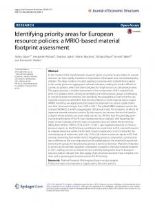
FIGURE 1

The bathymetry of the Eurasian sector of the Arctic Ocean with borders and boundaries used to define the search area

32

SOLOVYEV

ET AL.

however, use the term ‘network’ throughout the text emphasizing

water mass (the core of which has high salinity >34.5 psu) enters the

that this is yet not an ideal network derived from the theory of

Arctic in two ways: with the coastal current along the continental land

conservation biology.

in the Barents Sea, and from the north in the intermediate layer (100–

The purpose of this paper is to demonstrate how the methodol-

300 m) between Spitsbergen and Franz Josef Land archipelagoes, in the

ogy of identification of CPAs could be applied in the Arctic and

troughs of the northern Kara Sea, and in the Laptev Sea slope (Dmitrenko

examine a possible configuration of a network of priority areas for

et al., 2006; Rudels, 2015; Seidov et al., 2015; Zalogin & Kosarev, 1999).

conservation in the Arctic seas, which is a vast, poorly studied, highly

The water masses of the Siberian shelf, strongly influenced by

dynamic region for which only sparse data are available and to draw

river discharge consist of two cores (river runoff derived waters)

some practical lessons for future planning of the conservation efforts

bounded by the 25 psu isohaline: in the Kara Sea at the mouth of

both in the Polar Regions and in the High Seas.

the rivers Ob’ and Yenisei, and in the Laptev and East Siberian seas. The maximum expansion of the freshened water masses takes place

2 EURASIAN ARCTIC SEAS ENVIRONMENT A N D BI O G E O G R A P H Y |

in summer while the minimum is observed in late winter; there is also significant variation related to meteorological situations (Bauch, Dmitrenko, Kirillov et al., 2009; Bauch, Dmitrenko, Wegner et al.,

Russia's internal marine waters, territorial sea, the EEZ and the conti-

2009; Dobrovolsky & Zalogin, 1982; Seidov et al., 2015; Zalogin &

nental shelf encompass most of the Eurasian Arctic seas except the

Kosarev, 1999; Zatsepin, Kremenetskiy, Kubryakov, Stanchny, &

western Barents and the Norwegian Seas (Figure 1). The Barents, Kara,

Soloviev, 2015).

Laptev, East Siberian and Chukchi shelf seas, and the semi‐landlocked

The Pacific water mass is best defined by the 0°C surface

White Sea are part of the Arctic Ocean. The Bering Sea belongs to the

isotherm in June before the water column warms up in summer. In

Pacific Ocean. The boundaries of the Eurasian Arctic seas are demar-

winter

cated by conventional borders or by the islands and archipelagos. Most

(Dobrovolsky & Zalogin, 1982; Rudels, 2015; Seidov et al., 2015;

of the Eurasian Arctic sea area (and in some cases entire seas) is located

Zalogin & Kosarev, 1999).

on the continental shelf where water depth exceeding 200 m is not common (except for the Barents and the Laptev Seas) (Figure 1). The Eurasian Arctic seas represent an open area where four core water masses are advected from the outside (Figure 2). The Atlantic

FIGURE 2

this

water

mass

undergoes

complete

transformation

The distribution of the Arctic water mass is defined by the −1°C surface isotherm. This water mass is characteristic for the circumpolar Arctic Ocean (Dobrovolsky & Zalogin, 1982; Rudels, 2015; Zalogin & Kosarev, 1999).

Location of core water masses (A, C, D, E, P) and the main frontal areas (A/C, D/B, D/C, E/C, P/C) and particular types of transformed waters (at, Ct, W) in the Eurasian sector of the Arctic Ocean. Schematic map prepared by Pantyulin and Chuprina (2015) based on Boyer et al. (2012) A/C – Atlantic and Arctic water frontal area, D/B – Barents Sea and river runoff derived water in the Kara Sea frontal areas, D/C – Arctic and river water in the Kara Sea, E/C – Arctic and river runoff derived water in the east Siberian and the Laptev seas, P/C – Pacific and Arctic water, At – Transformed Atlantic waters, Ct – Transformed Arctic waters, W – White Sea waters. Transformed coastal water masses are not shown

SOLOVYEV

33

ET AL.

Water masses of particular seas undergo various transformations.

landfast ice that forms specific marine habitats (Carmack et al.,

Frontal transformation in the areas of contact between core water

2006). The extent of landfast ice varies significantly in different

masses is of particular importance for the purpose of this study. In this

regions, ranging from tens of metres to hundreds of kilometres

regard the frontal zone between the Atlantic and Arctic waters, i.e. the

(Figure 3).

so called Polar Front can be defined using both temperature and

Flaw polynyas are extensive areas of open water or of new unsta-

salinity gradients (Figure 2 A/C) (Dobrovolsky & Zalogin, 1982; Loeng,

ble ice that are regularly formed in particular areas during the winter

1991; Rudels, 2015; Seidov et al., 2015; Zalogin & Kosarev, 1999).

season between landfast ice and close pack ice (Figure 3). The

The frontal zone between the waters influenced by river discharge

polynyas in the Siberian shelf are formed as a result of specific atmo-

and the Arctic waters is defined using steep gradients of surface salin-

spheric processes, in particular regular winds pushing drifting ice off-

ity (between 25‰ and 30‰). Two such zones are delineated. The

shore (Popov & Gavrilo, 2011; Zakharov, 1996). Zakharov (1966,

western one is the contact area of the Ob’–Yenisey waters and the

1996) called polynyas ‘ice factories’, highlighting the fact that up to

Arctic waters in the Kara Sea (Figure 2 D/C), defined for the purposes

70% of the total volume of sea ice developing in the Arctic seas may

of the present study as the Kara Front. The eastern one is located in

be produced in polynyas. In spring and in summer polynyas accumulate

the northern part of the Laptev and East‐Siberian seas where the Lena

heat and become centres of seasonal sea ice decay (Zakharov, 1966,

and Indigirka rivers water contacts the Arctic water mass (Figure 2 E/C)

1996). They are considered to be extremely important for the Arctic

(Bauch, Dmitrenko, Kirillov et al., 2009; Bauch, Dmitrenko, Wegner

marine biodiversity and ecosystem (Carmack et al., 2006; Kupetsky,

et al., 2009; Dobrovolsky & Zalogin, 1982; Zalogin & Kosarev, 1999).

1961; Spiridonov, Gavrilo, Krasnova, & Nikolaeva, 2011).

The contact zone between the Pacific and the Arctic waters (Rudels,

In the last two decades there were hardly any areas in the Eurasian

2015) is located in the northern Chukchi Sea (Figure 2 P/C). It can be

Arctic seas where high concentrations of multiyear sea ice persisted

defined by the summer surface temperature.

from year to year; furthermore most of the Eurasian Arctic seas

In addition, there are transformed water masses which bear

became ice free by September (Frolov, Gudkovich, Karklin, Kovalev,

unique characteristics, i.e. the Barents Sea water (cooler than the

& Smolyanitsky, 2009; Jeffries, Richter‐Menge, & Overland, 2015;

Atlantic water mass but retaining the high salinity of the latter)

Maslanik, Stroeve, Fowler, & Emery, 2011). However, in particular

(Dobrovolsky & Zalogin, 1982; Loeng, 1991; Zalogin & Kosarev,

areas sea ice massifs can persist during sea ice decay thus maintaining

1999) and the smaller areas of particular bays, straits (Pantyulin,

marginal ice zone conditions for a prolonged time and influencing pro-

2012) and troughs (Zatsepin, Poyarkov et al., 2015).

ductivity and other ice related processes (Gavrilo & Spiridonov, 2011).

While the western and the south‐western parts of the Barents Sea

Biogeographic regionalization of the Russian Arctic may be well

are ice‐free all‐year round because of the inflow of the Atlantic water,

represented by respective schemes for macrozoobenthos (Petryashov

other Russian Arctic waters freeze in winter. Significant parts of the

et

coastal zone of the Russian Arctic seas are seasonally covered with

Redkozubov, & Petryashov, 2015). This regionalization system is in

al.,

2010,

2013;

Spiridonov,

2011;

Spiridonov,

Vedenin,

FIGURE 3 Location of landfast ice and flaw polynyas in the Eurasian Arctic seas (excluding the Bering Sea) in 2000–2015 mapped on the basis of satellite images (Dobrynin, 2015)

34

SOLOVYEV

ET AL.

many respects similar to the scheme of ichtyogeographical regionaliza-

Marine Ecosystems (AMAP/CAFF/SDWG, 2013 via ArkGIS, WWF's

tion (Chernova, 2011) and overlaps with the phytogeographic regional-

map portal for the Arctic). In the case of an overlap, the northern-

ization scheme for macroalgae (Zinova, 1974). Benthic biogeographic

most border was selected. The south‐eastern boundary of the

boundaries reflect the influence of environmental factors at different

research area was on the Navarin Cape latitude in the Bering Sea

spatiotemporal scales while planktonic boundaries are in many ways

to the south of the Anadyr Bay and the Chirikov Basin as this is

similar but usually have higher spatial resolution (Mokievsky, 2009).

where the border between temperate Northern Pacific and Arctic

Main biogeographic provinces roughly correspond to distribution of

realms lies (Spalding et al., 2007). On land the research area was lim-

core water mass. The Eurasian Arctic Province is associated with the

ited by the sea–land border, though technically it expanded inland,

Arctic water mass and the Atlantic water mass in deeper layers; the

the land‐based units were disregarded in the analysis (Figure 1).

Amerasian Arctic Province corresponds to the Arctic water not under-

The estuaries of the biggest rivers (the Ob’ and the Yenisei rivers)

laid by the Atlantic water; the Siberian Shelf Province reflects the influ-

were included in the research. Total area of research was over 6

ence of the river runoff derived water. The advection of the Atlantic

million km2, which is 2.5 times bigger than the Mediterranean Sea.

water in the Barents Sea and the Pacific water in the Chukchi Sea

The Lambert azimuthal equal‐area projection with central meridian

are reflected in the extensive biogeographic transitional zones in the

100°E based on WGS84 ellipsoid was used.

Barents and the Chukchi–East Siberian Seas. Distinct biogeographic districts are present in the White Sea and some other coastal areas owing to peculiar oceanographic conditions, including freshwater influ-

3.2

|

Environmental characteristics in the analysis

ence, and sea ice regime (Naumov, 2001; Petryashov et al., 2010;

The bathymetric conditions of the Eurasian Arctic seas are diverse and

Spiridonov, 2011; Spiridonov et al., 2015).

contrasting (Figures 1 and 2). Bathymetry data were often used as surrogates of benthic habitats (Table 1; Supplementary material).

3

METHODS

|

The study was based on existing data, both published and unpublished (e.g. remote sensing data). MARXAN software (Ball & Possingham, 2000) was selected as a decision support tool to structure and process data and assist experts in identifying the high conservation priority areas. The research was conducted by a team of experts from a number of Institutes of the Russian Academy of Sciences, the leading Universities and research centres and coordinated by the WWF Russia. The work was organized around a series of workshops. In between meetings experts continued to work individually and in groups. The main phases of the research included: 1. Defining basic parameters of the analysis: area of research, scale of processes and units and conservation features. 2. Collection, validation and compilation of data and definition of targets.

Polynyas, fast ice, areas of icebergs distribution and high concentration of multiyear ice zones were mapped using remote sensing data. Images produced by various satellites were used: LANDSAT‐5, LANDSAT‐7 (2005–2015, 563 images processed and 43 decoded), AMRSE, AMRSE‐2 (2000–2014, over 7000 images processed and 208 decoded), MODIS‐TERRA, MODIS‐AQWA (2007–2015, 784 images processed and 51 decoded). Mapping was done at 1:500 000 scale using Mapinfo v 8.2 Scanex Geomixer v 2.31, Scanex Image Processor v. 4.25.1 software. The spatial distribution of results of the supervised classification was used for preparing learning data for different spectral bands. Estimated signatures were used for seasonal mapping with post‐process verification of accuracy. Regions with prevailing distribution were selected (Dobrynin, 2015). Information on polynyas, extensive landfast ice areas (Figure 3) or areas of prolonged conditions of the marginal ice zone (MIZ) were used directly to define conservation features (CFs) or as surrogate data for inferring biological CFs, such as wintering areas of Laptev Sea walruses

3. MARXAN analysis and calibration of its parameters.

(which can hardly be found outside polynyas since this population does

4. Post‐MARXAN analysis, expert verification and interpretation of

not leave the Laptev Sea in winter). Major frontal zones were defined on the basis of the NOAA

results.

Arctic Regional Climatology atlas (by Boyer et al., 2012; Seidov Research was done in 18 months from the first meeting to the presentation of the final results.

et al., 2015; see Figure 2, Table 1). The frontal zones and the multiyear ice zones contributed to decreasing the cost of cells in the MARXAN analysis (see 3.9 Cost Layer).

3.1

|

Research area

The research covered those parts of Arctic seas under Russian juris-

3.3

|

Selected scale of processes and units

diction: the eastern part of the Barents Sea, the White Sea, the Kara

The research area was divided into 6674 planning units (PUs) –

Sea, the Laptev Sea, the East‐Siberian Sea, the western part of the

square cells with a side length of 30 km. This scale was determined

Chukchi Sea and the north‐western part of the Bering Sea

by the quality of data available for analysis and the scale of pro-

(Figure 1). The research area on the east and the west was limited

cesses under analysis. For the purpose of unification and compila-

by borders with Norway and the USA respectively. The northern

tion, all vector data layers of different quality were transformed

boundary of the research area was the edge of the Russian exclusive

into a raster on the more detailed grid composed of 5 × 5 km cells

economic zone (EEZ) and the northern limits of the relevant Large

nested into the 30 × 30 km network.

SOLOVYEV

TABLE 1

35

ET AL.

Criteria for selection of conservation features and examples

General criterion

Examples of specific conservation objectives

Number of CFs

Protection of rare communities of Zostera, especially in the Arctic seas outside the White Sea

16

Zostera communities, Ramsar zones, polynyas

Special importance for life‐history Protection of breeding/foraging, feeding ranges and stages of species migration corridors of particular rare species and species maintaining ecosystem functions and structures

72

Arctic cod spawning grounds, gray whale summer concentrations

Importance for threatened, Protection of ranges of species listed in IUCN red endangered or declining species list and Russian red data book and/or habitats

44

Ivory gulls colonies, Atlantic population bowhead whale range, Greenland shark range

Vulnerability, fragility, sensitivity or slow recovery

Protection of walrus rookeries at the seasons when walruses are present there

15

Laptev walrus rookeries, sponges concentrations

High biological productivity

Protection of areas of high productivity in the marginal ice zone

13

Kittiwake and Brünnich's guillemot wintering areas, marginal ice zone

High biological diversity and naturalness

Protection of areas of high benthic diversity associated with kelp communities

12

Matochkin Shar Strait kelp community, Zostera communities

Representativeness

Protection of a share of each phytogeographic region in the Russian Arctic seas

79

Trenches of the Kara and Barents Seas brackish waters communities, Eurasian province of Arcto‐Atlantic phytogeographic region

Genetic diversity

Protection of each geographical population of kittiwake/protection of kittiwake ranges in each of the Russian Arctic seas

65

Distribution of kittiwake in the Barents Sea, Macoma calcarea communities

Maintenance of ecosystem functions/structures

Protection of habitats/ranges of common, abundant species of birds

79

Common eider range, ringed seal habitat preference, polynyas

33

Nawaga spawning grounds, Pacific walrus whelping patches

Uniqueness or rarity

Areas/species important for local, Protection of habitats of marine mammals hunted by including indigenous population indigenous population of Chukchi region

3.4

|

Conservation features: Criteria for selection

Examples

invertebrates was also used for a general assessment of biogeographic representativeness of the resulting CPAs network.

For the purpose of the project, conservation features (CFs) were iden-

Types of habitat were defined by geomorphological (i.e. bottom

tified as spatially definable components of biodiversity and ecological

topography, coastline), sedimentological and oceanographical (includ-

processes, such as species and populations ranges, key habitats, com-

ing tidal regime and polynyas) characteristics. In addition, several CFs

munities' biotopes and locations of special zones/features. Conserva-

representing specific benthic communities dominated by one or sev-

tion features were selected in a broad context (Ball, Possingham, &

eral macroinvertebrate species and distributed over extensive areas

Watts, 2009). The following criteria for ecologically and biologically

were selected (Denisenko, Sirenko, Gagaev, & Petryashov, 2010; Kiyko

significant areas (EBSAs) were used to select conservation features:

& Pogrebov, 1997; Petryashov et al., 2010).

uniqueness or rarity, special importance for life‐history stages of

Distinctive benthic CFs included areas with increased benthos

species, importance for threatened, endangered or declining species

biomass at the scale of a particular sea, some remarkable systems of

and/or habitats, vulnerability, fragility, sensitivity or slow recovery,

benthic habitats such as fjordic lagoons and communities, seagrass

biological productivity, biological diversity and naturalness (Skjoldal &

meadows that seldom occur in the Arctic and endemic kelp of the

Toropova, 2010; UNEP/CBD/COP/DEC/IX/20, 2008). To achieve

Matochkin Shar Strait in Novaya Zemlya (Flerov, 1932). Areas with a

the goal of the project four additional criteria were added: representa-

high concentration of indicators of vulnerable marine ecosystems

tiveness, genetic diversity (representativeness at the population level),

(VME as defined by the FAO (2009)) that occur in the Barents Sea,

maintenance of ecosystem functions/structures, and areas/species

the White Sea and the Kara Sea were also included as separate CFs.

important for indigenous peoples (Table 1).

Conservation features for vertebrates were presented as spe-

Experts independently selected CFs for benthos, fish, seabirds and

cies ranges in general, i.e. for keystone, common and abundant,

marine mammals (for sources of data see Table S1) (Table 1) and then

commercial and endangered, threatened or protected (ETP) species

discussed and corrected the lists during a series of workshops and

of fish, mass and ETP species of seabirds and marine mammals

through MARXAN analysis.

and as distinctive parts of their distribution ranges such as breed-

Benthic CFs were selected primarily to represent biogeographical units and habitat types. They therefore included biogeographic

ing, foraging and other important areas (mostly for vertebrates) (Table 1; Table S1).

provinces as spatial proxies of flora (for macroalgae, Zinova, 1974)

Several CFs were defined for some species. For instance, there are

and fauna both for benthic invertebrates (Petryashov et al., 2010,

three different populations of walruses in the research area and their

2013; Spiridonov, 2011; Spiridonov et al., 2015) and fish (Chernova,

haul‐out sites and whelping patches were counted as separate CFs

2011). The present biogeographic regionalization scheme for benthic

with specified amounts, weights, targets and other parameters.

36

SOLOVYEV

ET AL.

Conservation features covered different levels of biodiversity.

opinions. Both direct data on CFs distribution and its surrogates were

Several CFs related to particular and often specific populations of cer-

used for analysis, e.g. data on fast ice distribution were used as a

tain species thus covering the population level, i.e. the particular pop-

surrogate for the distribution of ringed seal whelping patches.

ulations of the Atlantic salmon, the common eider, the beluga whale,

Metadata describing data sources, methods of collection, quality, time

the Atlantic and Pacific walrus and different populations of the polar

period and other characteristics for each dataset were also collected

bear. This situation mostly applies to vertebrates but also to the geo-

(Table S1).

graphically separated populations of seagrass (Zostera marina). For most of the selected seabirds and marine mammals, as well as for several fish species, the study aimed at conservation of species in the Arctic by protecting their habitats and thus covered the species level. At the community level entire areas hosting spatial complexes of different benthic and (indirectly) pelagic communities including those in fjords, fjordic lagoons, lagoons of accumulative origin, estuaries, shelf banks and troughs and coastal zones of archipelagoes were considered. Finally by inclusion of biogeographical regions the research considered the level of distinct floras and faunas (for macroalgae,

3.6

|

Data quality, gaps in data

Experts assessed the quality of each dataset as ‘low’, ‘medium’ or ‘high’ depending on data credibility that comprised data accuracy, method of collection, and time of data collection (Figure 4). Distribution of the number of layers and their quality per unit is presented on Figure 4. A Data Coverage Index was calculated as the number of layers multiplied by the quality index, with high quality datasets having index 3,

benthic invertebrates and fishes, see above).

medium – 2, and low – 1.

3.5

3.7

|

Data sources, types, and rejected data

|

Weights of datasets

Data on CFs distribution were presented as shape‐files; one shape‐file

All datasets were weighted for MARXAN analysis. The weight of each

per CF. Data were collected by experts on the region and taxonomic

CF was based on its data quality, number of objectives it met and type

groups.

of data it contained (surrogate or direct).

About 300 datasets were compiled; more than 80 of them were

Initially each dataset received the highest possible weighting –

rejected as inappropriate or redundant for the purposes of the

100. Then it was decreased according to criteria listed below

research and weren't used directly (Table S1 ‘Rejected data’). The

(Table 2). After a number of MARXAN tests some weights were

number of datasets used for MARXAN analysis varied from test to

adjusted by the expert team. All the changes of the weights were doc-

test; in the final test 195 layers were analysed.

umented (see Table S1). For example, Laptev walrus haul‐out sites on

Data were collected from different sources: direct field surveys, remote satellite surveys, modelling or as spatially presented expert

FIGURE 4

ice got weight 80, because the dataset quality was low, it satisfied five criteria and was based on results of field surveys – direct data.

Data coverage index distribution: Density of data layers used in analysis weighted by data quality

SOLOVYEV

TABLE 2

37

ET AL.

Weighting criteria for datasets

Quality

Number of criteria

Type of data

areas (Ball & Possingham, 2000). All data layers were created, orga-

Low

Medium

High

nized and processed as shape‐files using ArcGIS 9.2 (ESRI, 2006) and

−20

−10

0

QGIS 2.6.1 (Quantum GIS Development Team, 2014). ‘ESRI Shapefile’

1

2–3

>4

‐20

−10

0

Surrogate

Direct

‐10

0

format was applied for ‘points’, ‘lines’ and ‘polygons’ geometries. R package ‘rgdal’ was used to import/export ESRI Shapefiles (Bivand, Keitt, & Rowlingson, 2016). After that the data were prepared for MARXAN analysis: special scripts were written in the R programming language using GDAL library (GDAL, 2016; R Core Team, 2016). Other scripts for MARXAN analysis calibration and post‐analysis were also

3.8

Conservation targets

|

written using GDAL library.

As there is no solid scientific basis to access basic sufficiency of a conservation feature representation in the network of protected areas (Margules, Pressey, & Williams, 2002), the Aichi Target 11 (10%) was used as a basic conservation target (minimum share of a CF within the network of protected areas) (CBD, 2010). Doubled Aichi Target 11 (20%) was used as the conservation target for rare and unique species as well as for areas of special importance for life‐history stages of keystone species. After the first series of MARXAN tests and calibrations, experts decided to raise targets for some CFs, for example the target for Zostera communities outside the White Sea was set at 100%. All weights and targets are presented in Table S1.

3.11

|

MARXAN analysis

Repeated MARXAN runs were performed with different scenarios to define a range of options regarding the parameters and the location of potential priority areas. The team of experts reviewed the options proposed on the basis of MARXAN runs and eventually approved the final list by consensus. One of the benefits of MARXAN analysis is that it is an iterative process that can be repeated after data and parameters are added or corrected. Six full test cycles were conducted; results of each cycle were analysed during expert workshops. Each cycle included calibration and looked into a number of scenarios in search of conservation

3.9

Cost layer

|

priority areas. Calibration was intended to test certain technical param-

The cost of each PU was defined primarily by its area. Apart from area,

eters of the project including the number of iterations, boundary

particular oceanographic characteristics could influence cost of some

length modifier (BLM) and species penalty factor (SPF) (Ardron,

PUs. Coefficients lowering cost were set for the areas of major fronts

Possingham, & Klein, 2010; Ball & Possingham, 2000).

(which were used as surrogates for potential areas of high diversity and

The number of iterations was calibrated to identify the number

productivity) and for the areas of multiyear ice distribution (Table S1).

sufficient for MARXAN to provide an efficient solution. BLM regulated

Coefficients were defined after a series of MARXAN tests and calibra-

clumping of the solutions, while the SPF was used to determine the

tions by the expert team.

significance of CF individual weights in the analysis and helps MARXAN reach all project targets (Ardron et al., 2010).

3.10

|

Software

The optimal number of iterations was determined as 50 × 106. Optimal BLM and SPF were identified through calibration and visual

Geographic Information Systems (GIS) software and the decision sup-

analysis by the expert team and set at 0.3 and 0.04 respectively

port tool MARXAN were used to define and map conservation priority

(Figure 5).

FIGURE 5 Calibration of BLM and SPF used in Marxan project: A) in relation to the number of PUs (planning units) B) in relation to the missing values (CFs)

38

SOLOVYEV

TABLE 3

ET AL.

MARXAN analysis scenarios

Number

Name of the scenario

1

Basic: Normal targets, all CFs included in the analysis

2

Basic + existing PAs included in the analysis

3

Only existing PAs included in the analysis

4

Normal targets and basic parameters but only the CFs providing ecological functions included in the analysis

5

Normal targets and basic parameters but only the CFs representing rare and endangered species, populations, habitats and ecosystems included in the analysis

6

Normal targets and basic parameters but only the CFs providing representativeness functions included in the analysis

7

High targets scenario

By design MARXAN is not a decision‐making, but a decision‐

After all calibrations and corrections the following scenarios were used to determine the conservation priority areas (Table 3).

support tool (Ardron et al., 2010). In the project it was used to

Scenario 1 (Basic) was intended to show the distribution of

facilitate setting goals and targets, data handling and processing.

potential priority conservation areas. Scenario 2 showed the effi-

After six cycles of analysis the expert team considered the machine

cient distribution of these areas and took into account the existing

analysis sufficient. A broader team of experts then reviewed and

PAs. Outputs of these scenarios (total size of the conservation

corrected the configuration of the network proposed by MARXAN.

priority areas, number of targets achieved) along with outputs of

The team consisted of both experts that initially worked on the

Scenario 3 demonstrate the effectiveness of the proposed network

project and those that joined later. Results provided by MARXAN

in comparison with the existing PAs.

were carefully reviewed through a series of six workshops.

Scenarios 4–6 were intended to demonstrate to which of the

As a result the map of conservation priority areas was produced

criteria the selected areas mostly contributed: conservation of key-

(Figure 9) with lists of CFs supposed to be protected in each of 47

stone species providing ecological functions, protecting rare and

selected areas. For each selected area these CFs were ranked as ‘very

endangered species, or providing representativeness. The purpose

important’, ‘significant’ and ‘others’.

of Scenario 7 was to check if increasing targets would augment the size of originally selected areas or result in emergence of new priority areas.

4

3.12 | Post‐analysis: Ecological and geographical connectivity, representativeness, naturalness and stability

4.1

As MARXAN isn't able to fully incorporate the connectivity factor

Figure 7.

RESULTS

|

|

MARXAN analysis

Results of the final scenarios 1–7 are presented in Figure 6, with the basic scenario (Scenario 1) outputs presented in the more detailed

(Ardron et al., 2010; Roff & Zacharias, 2011), the assessment was per-

The total area of the best solution provided by MARXAN in the

formed by experts. They analysed ecological and geographical connec-

basic Scenario 1 was 771 924 sq km or 16.73% of the Russian Arctic

tivity for each of the CFs and made necessary corrections to the data

seas area. All 195 conservation targets were achieved in this solution

before the final runs. For the purpose of the research, connectivity

and most of them exceeded the minimum set targets (Figure 8). The

was interpreted as both an ecological and a geographical factor; the

resulting distribution of conservation priority areas showed that the

ecological dimension covered trophic connections, e.g. beluga whale

biggest areas were located in the central part of the research area.

and Arctic cod are supposed to be protected in the same area, while

Smaller but more numerous areas were located in the western and

the geographical factor accounted for connections between different

the eastern seas – the White Sea, the Barents Sea, western part of

habitats of the same species/population: feeding areas, whelping areas

the Kara Sea, the Chukchi Sea and the Bering Sea. The areas in the

and migration corridors between them.

East‐Siberian Sea were the smallest in size and number. Most of the

Another factor that experts analysed during the post‐analysis was

areas were attached to a shoreline or located in the vicinity of the shore.

representativeness. The aim of this exercise was to make sure that all

Results of additional Scenario 2 demonstrated that including

species and populations were presented in the selected areas of differ-

existing protected areas in a result ‘by default’, i.e. locking PUs within

ent geographical regions.

existing PAs into the output, only changed the configuration of

The criterion of naturalness was used to make sure that areas

selected PUs insignificantly by increasing the number of selected PUs

selected as important for CFs did not overlap with areas of anthropo-

in the areas around existing PAs. Total area of the best solution in this

genic pressure and that the most natural areas possible were selected.

scenario was 17.2% of the Russian Arctic seas which is just 0.5% more

The redundancy check was intended to make sure that each CF

than in the scenario where PAs are not taken into account. Only

was represented in at least two different areas, as that would provide

existing protected areas were included in the resulting configuration

additional protection in case of a disaster in one of the areas.

in Scenario 3.

SOLOVYEV

FIGURE 6

39

ET AL.

Results of scenarios (1–7) presented as distribution of PUs selection frequency

Scenarios 4 to 6 demonstrated to which criteria selected areas mostly contribute: conservation of keystone species providing ecological functions, protecting rare and endangered species, or providing representativeness. Some areas such as Franz Josef Land waters or

of the same archipelago that provides for conservation of rare features and species.

4.2

|

Conservation priority areas

the common outer frontal area of the Ob’ and Yenisey river mouths

Conservation priority areas that resulted from MARXAN and post‐

in the Kara Sea, generally ice‐free coastal areas of the north‐western

MARXAN analyses are presented in Figure 9. The breakdown of areas

part of the Kola Peninsula were selected as providing all three types

by particular marine basins and quantitative coverage characteristics of

of functions in a potential system of conservation priority areas. Most

the defined areas are summarized in Table 4.

of the areas contribute to two out of three: e.g. coastal waters of

The total size of the areas calculated through the experts' analysis is

north‐eastern Novaya Zemlya are important for conservation of key-

1 145 117 km2 or 24.8% of the Russian Arctic seas. Forty‐seven areas

stone and rare species and features, as well as the shallow shelf around

were identified. Their size varied from 96 to 88 920 km2 (Table 3).

the Lena River delta providing protection for endangered species and is important for representativeness of a potential network of MPAs.

Shares of CFs included in the network of conservation priority areas by far exceeded the previously established conservation

Some of the selected areas were significant only for one of the

targets: average target for a CF was established as 16.6% and

functional groups, like coastal waters of the Severnaya Zemlya archi-

included in the network as 36.6% (median is 20% and 30.85%

pelago that provides representativeness, or the area to the north‐east

respectively) (Figure 8).

40

FIGURE 7

SOLOVYEV

ET AL.

Distribution of proposed conservation priority areas, MARXAN: Scenario 1, PUs selection frequency

FIGURE 8 Distribution of conservation targets: Initial, achieved with existing PAs, achieved with MARXAN best result and the experts' choice conservation priority areas

5 | D I S T R I B U T I O N A N D SI Z E O F T H E PRIORITY CONSERVATION AREAS IN R E LA T I O N T O P A R T I C U L A R S E A S

areas in the Laptev Sea and the Bering Sea are also large. The CPAs in the White Sea are smaller than in any other sea including the smallest CPA in the entire Russian Arctic (96 km2). In spite of the differences between the seas, the total coverage of CPAs is

The greatest number of conservation priority areas (CPAs) was

roughly similar and for most seas is within the range 23–38%, or

identified for the Barents Sea (17) and the smallest for the Laptev

from a quarter to a third of the sea surface area. Only the East

Sea, Chukchi Sea and the north‐western Bering Sea (5) (Table 4).

Siberian Sea has a smaller coverage, at 16%. The CPAs of the

The Barents Sea was also characterized by the greatest range and

above‐mentioned seas have similar ratios of important and most

the largest of the areas (nearly 90 000 km2), while the smallest

important CFs.

SOLOVYEV

FIGURE 9

41

ET AL.

Conservation priority areas resulted from MARXAN and post‐MARXAN analyses

In the Barents Sea, areas 1–4 were nested within the generally ice‐

frontal area with frequent polynya events (26) and Baidaratskaya

free coastal realm of the Kola Peninsula representing different sea-

Guba (24) receiving less freshwater input. In the western part of

scapes, oceanographical conditions and biogeographical divisions

the sea, area 15 is located in the Kara front separating the Barents

along the direction of the peninsula coastal currents. Area 5 encom-

Sea and the Kara Sea waters in the St. Anna Trough and also includes

passes mostly shelf areas influenced by complex frontal systems on

the northernmost coastal areas of Novaya Zemlya. Area 25 encom-

the boundary between the Barents and the White Seas. Areas 21–23

passes fjords of the eastern coast of Novaya Zemlya, the deep and

are coastal areas of the shallow south‐eastern part of the Barents

narrow Matochkin Shar Strait separating the north and the south

Sea and cover most of the bays having various oceanographic and

Islands of the archipelago, and the eastern Novozemelskiy Trough.

sea ice characteristics. Areas 16, 17 and 19 are coastal areas of the

In the east, extensive areas represent the eastern shallow shelf of

west coast of Novaya Zemlya Archipelago with its skerries and various

the Kara Sea with numerous islands, a long lasting sea ice season

types of fjords. Areas 18 and 20 are representative areas of the eastern

and extensive fast ice (31), the waters of the Severnaya Zemlya archi-

Barents shelf with its banks (in particular Geese Bank) and troughs

pelago with associated fast ice and polynyas (30), and the area of

influenced by cold inflow from the Kara Sea (18), convergence of cold

Voronin Trough and the Kara Sea slope (29).

and warm currents and local upwelling (20). Area 12 represents

In the Laptev Sea the analysis resulted in selecting four areas.

troughs and banks of the northern Barents Sea and a characteristic

The western most area (32) covers the coastal zone of the east

segment of the Polar Front, while areas 13 and 14 reflect conditions

coast of Taymyr Peninsula and the western part of the Great

of waters around most high latitude Arctic archipelagoes in the

Siberian Polynya; the central area (33) is located on the shallow

Eurasian sector, Franz Josef Land (with Victoria I.) along with adjacent

shelf around the Lena River delta, also overlapping with part of

shelf and slope. The size of areas in the Barents Sea generally increases

the Great Siberian Polynya region. The eastern areas (34, 35) are

from the coastal to offshore zone and from the south to the north, with

located on the border between the Laptev and the East Siberian

areas 12 and 13 being among the largest selected areas.

seas to the north of the New Siberian Islands, also covering

The White Sea is represented by the areas which reflect a high variety of CFs over this relatively small marine basin. Areas 6, 9, and

polynyas and the waters around the most remote small high Arctic islands (De Long Islands in the East Siberian Sea).

11 encompass important structural divisions of the sea: Gorlo, the

Other conservation priority areas are located in the east of the

strait connecting its outer and inner parts (6), the deep Kandalaksha

East Siberian Sea. They include most of Chaun Bay (Chaunskaya Guba)

Bay with internal trough (9) and shallow Onega Bay with the Solovki

(36) and De Long Strait (39) along with the coastal zone and shallow

Archipelago (11). Areas 7, 8, and 10 are smaller coastal areas associ-

shelf areas around Wrangel Island in the boundary area with the

ated with particular bays and lagoons.

Chukchi Sea. In the Chukchi Sea proper the analysis revealed two

In the Kara Sea, shallow coastal areas represent the huge estuarine systems of Ob (27) and Yenisei (28) with their common outer

extensive shelf areas in the north (40) and the east (42) of the sea and a large coastal lagoon area of Kolyuchinskaya Guba (41).

42

*Calculated only for geographical boundaries of the seas. Area %: area as share of the area of a particular sea or two neighbouring seas; N CFs: number of most important and important CFs per area (min/max); AvN CFs: average number of most important and important CFs per area (SD). As several CPA cover parts of different seas, separate calculations were done for a particular seas and the neighbouring seas.

9 (6.01) 6–23 38 4086–33129 43,44,45,46,47 5 Bering

9 (3.85)

17 (5,95) 4–21 27 582–31048 38,39,40,41,42 5 Chukchi

10.5 (3.74) 7–18

7–18 11

16 1050–61057

1050–61057 34,35,36,37,38,39

29,30,32,33,34,35,36,37,38,39 10

6 East‐Siberian

Laptev and east‐Siberian

11 (3.07)

8 (4.47) 3–23

7–15 23

25 1027–83217

4190–55300 29,30,32,33,34

13,15,24,25,26,27,28,29,30,31,32,33,34 13

5 Laptev

Kara and Laptev

7.5 (5.95)

7 (4.98) 3–23

3–23 27

27 245–88920

1027–68416 13,15,24,25,26,27,28,29,30,31

1,2,3,4,5,12,13,14,15,16,17,18,19,20,21,22,23,24,25,26,27,28,29,30,31 25

10 Kara

Barents and Kara

10.5 (4.94)

7 (5.29) 3–23

6–21 33

27 245–88920

96–12377 5,6,7,8,9,10,11

1,2,3,4,5,12,13,14,15,16,17,18,19,20,21,22,23 17

7 White

Barents

Area IDs (Figure 9). Number of CPAs Sea

TABLE 4

Selected conservation priority areas (CPA) in particular seas and boundary areas*

Size range (km2)

Area %

N CFs

AvN CFs

SOLOVYEV

ET AL.

In the Russian part of the Bering Sea the entire western part of the Bering Strait was selected (43) along with the coastal zone of the southern Chukotka Peninsula including the region of Sireniki polynya (44). Other contrasting areas are the Anadyr Liman with estuarine conditions (47), extensive shelf area of the Gulf of Anadyr (45), and the Navarin Cape area (46) which includes various coastal lagoons and part of the Northern Bering Sea front.

6 | R EP RE S E N T A T I V E N E S S O F T H E S E L EC T E D N E T W O R K I N R E L A T I O N T O B I O GE O G R A P H I C A L U N I T S This was assessed using a regionalization system for benthic invertebrates (Petryashov et al., 2010, 2013; Spiridonov, 2011; Spiridonov et al., 2015) which is the most developed biogeographical regionalization scheme for the Eurasian Arctic (Table 5). Table 5 summarizes

the

representation

of

particular

biogeographical

regions in the network of conservation priority areas. All biogeographical units were represented in all relevant seas except the Amerasian Arctic province in the Chukchi Sea. That said, this province in the Chukchi Sea is located in the north and largely outside Russia's EEZ (Petryashov et al., 2013). Targets for representation of particular large biogeographical regions were not specified for particular seas but for the Russian Arctic in general. In spite of this, such large regions as the North Atlantic/Arctic transitional zone, Eurasian Artic Province and the Siberian Shelf province were represented by several large areas in all relevant seas (Table 5). Furthermore these areas capture distinct parts of respective biogeographical regions. For example the North Atlantic/Arctic transitional zone was represented by a series of coastal priority areas reflecting a gradient of species assemblages along the Murmansk coastal current direction (2–4), the western coast of Novaya Zemlya (16, 17, 19), the unique boreal refugium in the Chioshkaya Bay (21), and the bays of the White Sea with different conditions and associated fauna (6–11), along with offshore areas in different sections of the Polar Front (12, 18). The Siberian Shelf province is represented by transitional areas in the very south‐east of the Barents Sea, an enclave in the White Sea trough and areas with different levels of influence from estuarine waters in the Kara and the Laptev Seas. The Eurasian Arctic province was represented by the several areas in the north of the Barents and Kara Seas but could be underrepresented in the Laptev Sea (Table 5). Several areas cover the boundary zone between the Eurasian Arctic and the Siberian Shelf province (15, 30, 35). Finally, the transitional zone between the Arctic and North Pacific realms was represented by several areas in the Chukchi Sea and the refugium in Chaun Bay in the East Siberian Sea (36). Northern outposts of non‐Arctic biotas were selected in the south‐west of the Barents Sea (part of the Scandinavian province, 1), in the south of the Chukchi Sea (42) and in the north‐western Bering Sea (43–47).

6.1

|

Overlapping with existing protected areas

The total size of the existing protected areas is about 127 000 km2 or less than 3% of the total research area, thus they achieve conservation targets for only 36.4% of selected CFs (Table 5).

43

ET AL.

Bering

43–47

Results of the basic scenario of MARXAN analysis (Scenario 1, Figures 6, 7) show that the total area that needs to be protected to

32, 33, 34, 35 (part)

slightly bigger area – almost 793 000 km2 (17.2% of the Russian Arctic

42 (part)

39–41, 42 (part)

with existing PAs included (i.e. Scenario 2, Figure 6) demonstrate only a seas area) (Table 6). Most of the existing federal nature protected areas of the Russian Federation overlap with selected conservation priority areas

36 (part)*

(Figure 10). Overlapping is observed in the areas of the largest currently protected areas in the Russian Arctic seas: the Franz Josef Land area of the Russian Arctic National Park with area 13, and the Wrangel Island Zapovednik (strictly protected reserve) with area 39. The Kolyuchinskaya Guba (area 41) and parts of area 43. Some other important areas include small coastal zones of several federal reserves.

30 (part)

The total area of overlap of conservation priority areas with marine area of federal nature protected areas is 105 489 km2 or 83.05% of the total area of existing protected areas or 11% of conservation priority areas.

15 (part), 29, 30 (part)

24, 25, 31, 15 (part), 30 (part) 6–8, 10–11, 9 (part)

km2 or 16.7% of the Russian Arctic seas. Results of the basic scenario

recently established National Park Beringia includes most of the

26, 27, 28

Laptev Kara

7

|

DISCUSSION

7.1 | Comparison of the Russian Arctic case with other large‐scale systematic marine conservation planning efforts Systematic marine conservation planning is a relatively new field (Wells et al., 2016). However, there have been a few attempts to apply this approach to extensive marine areas, i.e. covering more than one sea or LME, which are comparable with the sector of the Arctic that

9 (part)

White

36 (part), 37, 38

35 (part)

36 (part)

E‐Sib

Chukchi

Not selected

achieve all the conservation targets should be no less than 772 000

Sea

the present study looks at. servation planning is rezoning of the Great Barrier Reef in Australia. In this project separate reefs were taken as planning units with buffer The most important CFs were 70 bioregions of particular types (both reef and non‐reef biotopes) derived from statistical modelling and 12 (part), 13, 14

expert analysis. The cost of a unit was a function of various human interests (i.e. fishing, recreation, use by indigenous people, and conservation) (Ball et al., 2009; Fernandes et al., 2005). *Chaun Bay refugium (Petryashov et al., 2010)

Transitional North Pacific/ Arctic zone

North Pacific realm

Conservation Law Foundation of USA (CLF) and WWF Canada ini-

Amerasian Arctic Province

Eurasian Arctic Province

23 Ob‐Yenissean Province

Siberian Shelf Province

5 (part), 12 (part), 18, 20

zones and the spaces between them divided into equal hexagons.

AATZ offshore

1

2–4, 5 (part), 16, 17, 19, 21, 22 (part) Atlantic/ Arctic transitional zone (AATZ) coastal

Scandinavian province

Barents

The classic example of how MARXAN can be used for marine con-

Biogeographical region

TABLE 5 Breakdown of selected areas of high conservation priority (as numbered in Figure 9) by major biogeographical regions (Petryashov et al., 2010, 2013; Spiridonov, 2011; Spiridonov et al., 2015) in particular seas. Grey: Non‐applicable

SOLOVYEV

tiated a project of systematic MPA planning of the Atlantic shelf of Canada. Although smaller in geographical extent this project had similar aims to the current study. The following groups of CF were used: areas of persistently high chlorophyll concentration obtained using Sea WIFS satellite images, demersal fish species richness in the bottom trawl surveys, adult and juvenile fish abundance, cetacean abundance, and habitat types classified from abiotic data, benthic and water characteristics (CLF/ WWF, 2006; Roff & Zacharias, 2011). The targets were set at 20% of high chlorophyll concentrations within the planned units, 20% of species richness or relative abundance contained in planned units at or above the mean for biogeographical area, and 20% of each seascape type. All planning units were assigned the same cost.

44

SOLOVYEV

TABLE 6

ET AL.

Parameters comparison of existing PAs in the Russian Arctic seas with the outputs of MARXAN analyses Total area, km2 (percentage of the total working area)

Conservation targets achieved (share of the total number of targets)

1. Basic: Normal targets, all CFs included into analysis

771 924 (16.73%)

195 (100%)

2. Basic + existing PAs included in the analysis

792 913 (17.19%)

195 (100%)

3. Only existing PAs included in the analysis

127 014 (2.75%)

71 (36.4%)

MARXAN scenarios

FIGURE 10

Overlapping of selected conservation priority areas with existing marine protected areas in the Russian Arctic

The largest marine region ever explored for conservation planning

(2015). Adding productivity characteristics would increase this number

using MARXAN prior to the current study was the North‐east Atlantic

by an order of magnitude. Statistical modelling and extensive expert

(the High Sea area outside the regional seas and EEZs of coastal states)

evaluation could reduce this number but for such a huge area as the

(Evans, Peckett, & Howell, 2015). This analysis used combinations (e.g.

Russian Arctic seas it would require an enormous amount of prelimi-

water masses plus seafloor kinds) of types of habitats and areas of high

nary work, much more than in the case of the Great Barrier Reef. In

physical diversity as a surrogate for biological diversity. The planning

addition, research would have to take into account a number of CFs

units were ICES statistical rectangles measuring 30 min latitude by 1

covering vertebrate populations not necessarily coinciding with biore-

degree longitude and thus the exact area in km2 varies with longitude.

gions as well as distinctive entities (such as VMEs).

The study by Evans et al. (2015) was mostly concentrated on achieving

Owing to time constraints and limited financial resources it was

efficient representation of habitat types and played therefore with dif-

decided to set aside this approach; however, it was noted that it was

ferent scenarios with varying conservation targets and BLM.

needed in order to perform a comprehensive assessment and deserved

All the above‐mentioned studies including the current one used

to be considered in the future. Instead, MARXAN was set to freely

very different approaches to the selection of habitat and conservation

combine particular habitat features even though they could be partly

features. The North‐east Atlantic and the Great Barrier Reef projects

overlapping (i.e. bathymetric zones, sediment classes and widespread

dealt with bioregionalization schemes. Unlike them, the study of the

types of benthic communities). This increased the likelihood of achiev-

Russian Arctic seas was not based on a single regionalization scheme.

ing appropriate representativeness of habitats through MARXAN runs,

A rough calculation of simple combinations for bioregions identified

one way or another.

on the basis of bathymetry, geomorphological characteristics of the

Similar to the CLF/WWF study (Roff & Zacharias, 2011) the pres-

coastline and seabed, sediments, water masses and fronts, sea ice

ent attempt at conservation planning was grounded upon both

regimes and biotic composition for macrophytes would result in a

representation of biogeographical regions and habitats and the

few hundred thousand bioregions of the scale comparable with the

distribution of life forms and distinctive areas. In contrast to the iden-

one used in the studies by Fernandes et al. (2005) and Evans et al.

tification of priority areas for conservation by CLF/WWF Canada the

SOLOVYEV

45

ET AL.

oceanographical characteristics were not directly integrated in the CF

intense commercial fishing (Bohanov, Lajus, Moiseev, & Sokolov, 2013;

set, except for prolonged MIZ and flaw polynyas which themselves

Lajus et al., 2005; Shevelev, Sunnanå, & Gusev, 2011) and there are arti-

may correspond to biological entities. Instead they influenced the costs

sanal and small‐scale commercial fisheries in the White Sea (Lajus et al.,

of planning units.

2005; Spiridonov & Suprunenko, 2016; Stasenkov et al., 2011) and

While the conservation planning for the Atlantic shelf of Canada

some coastal areas in the Kara Sea (Ulchenko et al., 2016) and marine

and New England used CFs reflecting pelagic productivity (i.e. areas

hunting and fishing in Chukotka (Bogoslovskaya, Slugin, Zagrebin, &

of high chlorophyll concentration) the study of the Russian Arctic did

Krupnik, 2007), there have been no fisheries in most of the Russian

not. The reason for this is the extremely high variability of primary pro-

Arctic and it is uncertain if any fishery development is possible in the

duction characteristics in the water column of the Arctic seas both spa-

region. The coastal regions of the western Kola Peninsula in the Barents

tially and seasonally (Vetrov & Romankevich, 2009, 2011) and the lack

Sea and the White Sea are experiencing a surge of tourism which is

of comparable data for alternative sources of primary production such

poorly regulated (Spiridonov & Suprunenko, 2016), while other poten-

as sea ice flora and microbiota (Carmack et al., 2006; Ilyash & Zhitina,

tially attractive areas remain generally pristine. Some of them are still

2009; Romankevich & Vetrov, 2001). However, the inclusion of

new to vessel‐based cruise tourism.

polynyas and marginal ice zone, known for their impact on primary

While active production of natural gas is underway in the Yamal

production (Carmack & Wassmann, 2006; Carmack et al., 2006), and

Peninsula and construction of terminals and pipelines is progressing

indirect effects of decreasing costs of planning units in oceanographi-

(WWF Russia, 2016), in most of the Russian Arctic seas hydrocarbon

cal fronts known for enhancing the effect on biological productivity

exploration remains limited. However, there are vast areas licensed

and biomass concentration (Carmack & Wassmann, 2006; Flint,

for hydrocarbon exploration (Amiragyan, 2016; Rosneft, 2016) and

Poyarkov, & Soloviev, 2015; Sakshaug, 2004; Sakshaug, Bjørge,

taking them into account would seriously bias conservation priorities.

Gulliksen, Loeng, & Mehlum, 1994) made it possible to account for

Considering the above‐mentioned it is currently impossible to esti-

essential productivity features (Spiridonov et al., 2017).

mate the costs associated with multiple present and, more impor-

The important difference of the Russian Arctic conservation plan-

tantly, potential economic activities for a particular unit. However,

ning experiment from others that are comparable in scale using

such costs should be considered during the next step when system-

MARXAN applications to marine conservation priority areas was that

atic conservation planning is done at a finer scale for particular seas

the latter either considered mostly the coastal zone (Ball et al., 2009;

and their subdivisions. This will require developing a set of new

Fernandes et al., 2005) or excluded it from the analysis (CLF/ WWF,

layers based on current economic activity (i.e. industrial fishery in

2006) while in this study both inshore and offshore planning units

the Barents Sea, shipping, natural gas extraction infrastructure in

were considered. This was necessary because of the enormous influ-

Yamal Peninsula, closed military areas, traditional coastal activities,

ence that coastal processes have on marine biodiversity in the Russian

and tourism), as well as modelled expected activities, such as hydro-

Arctic including formation of landfast ice, polynyas, and river discharge

carbon development, new shipping routes and possible industrial

(Spiridonov et al., 2011). In addition, many important vertebrate spe-

fishing beyond the Barents Sea.

cies such as seabirds, walruses, ring seals and beluga whales, and anadromous and semi‐anadromous fishes use both offshore and inshore/ estuarine habitats.

7.2

|

MARXAN and post‐MARXAN analysis

Separate analysis of inshore and offshore parts of the study area

Despite the fact that MARXAN is the only decision support tool in

would undermine connectivity of the resulting network of priority con-

most of the projects. The final outputs are considered to be poten-

servation areas and thus make very little sense. Moreover coastal and

tial protected areas, and the borders of potential MPAs usually

offshore habitat features and CFs should be analysed over different

match the borders of the areas selected by MARXAN. By contrast,

spatio‐temporal scales (Mokievsky, 2009; Roff & Zacharias, 2011)

the present survey attached special importance to post‐MARXAN

which would result in very uneven distribution of size of selected

analysis. Comparison of the final configuration and MARXAN pro-

areas, i.e. relatively small coastal areas in the Barents and White Seas

posed areas (basic scenario 1) is shown on the map (Figure 11)

vs a huge area along the outer shelf and slope of the Kara Sea

and in Table 7).

(Table 4; Figure 8). The studies for the Great Barrier Reef (Fernandes

There are some notable differences between the two configura-

et al., 2005), the Atlantic shelf of New England and Canada (CLF/

tions of the network. The experts increased the total size of the area

WWF, 2006) and the High Sea of the North‐east Atlantic (Evans

from 771 924 km2 (16.73%) to 1 145 117 km2 (24.8% of the Russian

et al., 2015) all selected areas that were comparable in size, however,

Arctic seas area). Overlap between MARXAN proposed areas and

this might be an initial intention of the authors.

areas in the final configuration chosen by experts is about 80% for

Although human use is a critical factor for systematic conservation

the areas most frequently selected by the algorithm and just a little

planning, the present study did not consider the increased costs of

above 70% for the areas with selection frequency of 60%. The experts

establishing a conservation regime in the areas of economic interest.

also included some areas that were not chosen by MARXAN and

This makes it very different from the rezoning of the Great Barrier Reef

ignored some of the MARXAN proposals.

(Ball et al., 2009), which, according to its rationale primarily focused on human uses. Economic activity in the Russian Arctic remains very uneven. While a significant part of the Barents Sea is among the world's oldest sites of

In total 11 new areas were proposed, 27 areas resulting from MARXAN analyses had their shape changed and enlarged, for two areas the size was reduced and two areas proposed by MARXAN were excluded by the experts (Figure 11).

46

SOLOVYEV

FIGURE 11

TABLE 7

ET AL.

Comparison of the network of conservation priority areas proposed by experts with the outputs of MARXAN analysis

Comparison of the final configuration of the CPAs network and MARXAN proposed areas (basic scenario 1) Total size of the areas proposed by MARXAN, thousands km2

Total size of intersection of conservation priorities areas, thousands km2

Share from the total area, proposed by MARXAN, %

Selection frequency 60%

663.1

502.5

71.4

Selection frequency 80%

483.8

378.9

78.3

Selection frequency 95%

304.9

243.8

79.9

Best selection

789.0

547.1

69.3

PU

For example, Victoria Island (area 14) and the Chioshskaya Guba

Some enlargements such as the area to the north of Franz Josef

(21) in the Barents Sea, Zhelania Cape to the north of Novaya Zemlya

Land waters (area 13), or new areas like area 14 (Victoria Island waters)

archipelago (15), areas to the north of Novosibirskie Islands (34, 35),

weren't selected originally by MARXAN and were added by the expert

and the area around Navarin Cape (46) in the Bering Sea weren't pre-

team during post‐MARXAN analysis because of gaps in the data used

sented on the selection frequency map after the final MARXAN runs;

for the MARXAN analysis, that did not show specificity and unique-

these as well as some other areas were proposed by experts and

ness of these particular areas for the developing network. This was

subsequently recognized as areas of conservation priority.

the second commonest reason for correction of areas established by

Some areas were enlarged significantly: in the area to the north of the Franz Josef Land archipelago (13), the Baydaratskaya Bay (24), the

MARXAN analysis. There were seven cases where existing areas were corrected or new areas proposed for this reason.

Gorlo (6), and the area to the north of Chukchi Peninsula (42). For

In two cases experts decided to select different parts of areas than

some areas boundaries were partly changed, e.g. for the water around

were proposed by MARXAN. For instance, in the Laptev Sea an area of

Wrangel Island (39) and the area of the Lena River delta (33). Some

the Great Siberian Polynya to the north of Novosibirskie Islands (34,

areas chosen by MARXAN weren't included in the final network, the

35) was selected because its diversity and productivity was higher than

most significant was a large area in the Laptev Sea between Taymyr

in the central part of the Polynya as chosen by MARXAN, based on the

Peninsula and the Lena River delta.

criterion of representativeness for some of the communities on a

The changes to the boundaries of 23 areas (enlargements or partial changes of boundaries) were made because the areas defined by

particular benthic substrate, because that criterion was already met in other selected areas.

experts followed contour lines along isobaths or other natural bound-

Some areas were altered or added for sustainability reasons – for

aries. It is customary in Russia to define boundaries of protected areas

example, the Chioshskaya Bay (21) was added to the network partly

following natural lines instead of using regular geometric shapes as

because it, along with benthic communities representativeness, pro-

many countries do.

vides alternative grounds for moulting harp seals in the years when

SOLOVYEV

47

ET AL.

ice conditions in the White Sea are unsuitable (Svetochev, 2013).

one or two orders of magnitude and many are 103–104 km2 in size,

Others, like the areas to the south of the Bering Strait (44) along the

i.e. a minimal biogeographical unit (Mokievsky, 2009) or an ecoregion

shores of the Chukchi Peninsula between two patches proposed by

(Roff & Zacharias, 2011).

MARXAN, were selected for reasons of connectivity (Solovyev,

Roff and Zacharias (2011) define an ecoregion as an area of rela-

Zagrebin, Glazov, Litovka, & Kosyak, 2013). There are seven areas

tively homogenous species composition, which is likely determined

where original boundaries were changed for reasons of sustainability,

by the predominance of a distinct suite of oceanographical or topo-

representativeness and connectivity.

graphic features. Indeed, most priority areas are based on such fea-

All these changes made by experts were only possible due to the

tures (Spiridonov et al., 2017), although most of them with the

transparency of the MARXAN‐based approach to analysis. All inputs,

exception of polynyas were not included in MARXAN analysis. The

changes and corrections were documented which allowed external

proposed network of conservation priority areas in the Russian Arctic

experts who were invited at later stages to participate in a broader

seas would consist of seascape‐ to ecoregion‐scale units which repre-

team to analyse results and understand how different parameters

sent practically all currently defined biogeographical provinces

and data influenced the outcomes of specific runs.

(Table 5) and would include different types of bays and straits

MARXAN proved to be a very convenient decision support tool

(although apparently not all the types) and most archipelago areas.

instrumental for structuring data and the process of analyses, but

Further research and analysis on CFs might reveal that other parts

serious post‐MARXAN analysis is required to interpret and correct

of the region also deserve the status of conservation priority areas.

the outputs.

However, we believe that they would be relatively small, probably not exceeding 103 km2. Even large conservation priority areas in the Arctic are used by highly migratory species of fish, seabirds and marine

8

|

T HE P R O P O S E D N E T W O R K

mammals only for short periods during the year. Their prey, such as polar cod is not confined to the conservation priority areas either.

The existing set of federal specially protected areas in the Russian

Therefore analysing the level of connectivity (Roff & Zacharias,

Arctic seas was shaped by the history of their development, while

2011) of the network with particular reference to highly migratory

long‐term planning and analysis of the challenges of preserving

top predators, many of them being iconic species for the Arctic, is a

marine biological diversity played little significant role in their

separate task. The authors intend to conduct a further special study

formation (Spiridonov et al., 2012). However, more than 80% of

of this subject.

existing protected areas were selected on the basis of MARXAN

Another critical issue is the sustainability of the suggested net-

analysis. This indicates close association of the priority conserva-

work in the face of the changing climate. There are several scenarios

tion features on the coast (which primarily determined the estab-

of how ecosystems might change under the influence of the current

lishment of the existing protected areas) with conservation

trends, such as the increasing input of the Atlantic and Pacific waters

features at sea.

into the Arctic, decreasing summer sea ice cover, change in the propor-

It should also be noted that in recent years a number of large

tion of multi‐year ice and increasing average temperature (Alexander

protected areas were established around the protected areas on the

et al., 2013; Carmack et al., 2006; Fossheim et al., 2015; Hunt et al.,

Franz Josef Land and Wrangel Island which significantly increased

2016; Kedra et al., 2015; Laidre et al., 2015; Melnikov, 2008).

the size of area under protection (Spiridonov et al., 2012). However,

A possible way to account for these changes could be continuous

the present study shows that a large marine area containing numerous

modelling for all the CFs based on the changing factors and repeated

important CFs as well as a number of biogeographical regions in the

MARXAN analysis of all possible scenarios. This would be a very

Russian Arctic remains outside the federal system of protected areas

resource‐intensive and time‐consuming exercise but an extremely

and according to the Ministry of Natural Resources and Environment

important one since biodiversity indicators in most of the selected

of the Russian Federation the existing plans to establish new PAs in

areas are based on particular oceanographical and other environmental

the region do not address these concerns.

features (Spiridonov et al., 2017). Possible climate‐related changes of

The network of conservation priority areas proposed by the

underlying environmental features of the proposed priority areas could

present project would provide protection for large parts of Arctic seas.

also be discussed and explored. We therefore consider the proposed

Large areas covering 25–30% of all seas with the exception of the East

network to present a sound basis for future development of the

Siberian Sea (Table 3) were identified as conservation priority areas.

protected areas and marine spatial planning in the Arctic.

This proportion does not depend on the size of the area under analysis, but there is a certain correlation between the size of specific proposed areas and the size of the marine basins in which they are located (i.e. smallest area is located in the White Sea and the two largest are in the Barents Sea and the Kara Sea).

9 | C O NC L U S I O NS : L E S S O N S F R O M TH E P R E S E NT SY S T E M A T I C C O N S E R V A T I O N PL AN NI NG R E SE ARC H

Mokievsky (2009) discussed the spatial scales that are sufficient to protect various habitat and conservation features in the World Ocean. 2

2

The first attempt to apply systematic conservation planning to the

He considered the scale of 10–10 km to be appropriate for the

selection of protected areas in the Russian Arctic seas revealed that

protection of series of benthic communities or seascapes. Most of

the available data for this vast area comprising about one‐third of the

the priority areas identified in the present study exceed this size by

Arctic Ocean were unevenly distributed and highly heterogenous

48

SOLOVYEV

(Figure 2; Table S1). However, even these data were sufficient to identify, through a series of experts' consultations, a set of conservation features (CFs) that met the EBSA criteria. Thus the present dataset includes a list of representative and distinctive areas which could be modified as and when more comprehensive data are available. The present study presents an alternative approach to how MARXAN could be used as a decision support tool. In contrast with other large‐scale studies that applied an integrated habitat classification the present research used several independent habitat classifications in various combinations. Another difference is that oceanographical features such as water masses and fronts were used, not to define integral bioregions and CFs, but to adjust the cost of a unit, i.e. to reduce the cost for units corresponding to frontal systems. The primary lesson learnt from the present study is that the optimal way to use MARXAN as a decision support tool is to supplement software runs with repeated expert analysis of results and post‐ MARXAN analysis. This iterative procedure and post‐MARXAN analysis did not radically change the MARXAN‐proposed network but allowed the identification of a more balanced system of conservation priority areas spread rather evenly throughout the Russian Arctic seas (covering from 25 to 30% of the sea area). The system encompassed both offshore and coastal zones ranging from relatively small shallow coastal lagoons and fjords with distinct features to extensive areas covering various biotopes in the shelf and upper slope zones. The resilience of the resulting network to climate‐induced ecosystem changes and potential surge of economic activity in the region deserves further examination; so does the institutional basis for its implementation (i.e. as specially protected areas in a strict sense, marine spatial planning zones, fishery management areas, etc.). We believe that the suggested approach combining MARXAN and post‐MARXAN analysis and the resulting network could become the first step towards systematic planning of the marine priority conservation areas in the pan‐Arctic region. ACKNOWLEDGEMEN TS This project was initiated by WWF Russia and funded by Oceans 5 foundation, WWF Netherlands and WWF Russia. The authors would like to thank all experts participating in national and international meetings for their comments, review and ideas for this research. Without their input this project would not have been possible. The authors thank Olga Movsinskaya for her assistance in manuscript preparation and John Roff, Jan Ekebom and the third anonymous reviewer, and John Baxter the editor of the journal for their careful review that

ET AL.

(Eds.), Contribution of working group I to the fifth assessment report of the intergovernmental panel on climate change (pp. 3–30). Cambridge, UK: Cambridge University Press. AMAP/CAFF/SDWG. (2013). Institute of Marine Research (IMR). Bergen http://wwfarcticmaps.org/ Accessed on 25 December 2016 Amiragyan, A. (2016). Oil and gas in Russian Arctic. TEC v Rossii, 09, 35–39. (in Russian) Amstrup, S. C., Marcot, B. G., & Douglas, D. C. (2008). A Bayesian network modeling approach to forecasting the 21st century worldwide status of polar bears. In Arctic sea ice decline: Observations, projections, mechanisms, and implications (pp. 213–268). Ardron, J. A., Possingham, H. P., & Klein, C. J. (Eds) (2010). MARXAN good practices handbook, Version 2. Victoria, BC, Canada: Pacific Marine Analysis and Research Association. www.pacmara.org Ball, I. R., & Possingham, H. P. (2000). MARXAN (V1. 8.2). Marine reserve design using spatially explicit annealing, a manual. Ball, I. R., Possingham, H. P., & Watts, M. (2009). MARXAN and relatives: Software for spatial conservation prioritisation. In A. Moilanen, K. A. Wilson, & H. P. Possingham (Eds.), Spatial conservation prioritisation: Quantitative methods and computational tools (pp. 185–195). Oxford, UK: Oxford University Press. Bauch, D., Dmitrenko, I., Kirillov, S., Wegner, C., Hölemann, J., Pivovarov, S., … Kassens, H. (2009). Eurasian Arctic shelf hydrography: Exchange and residence time of southern Laptev Sea waters. Continental Shelf Research, 29, 1815–1820. Bauch, D., Dmitrenko, I. A., Wegner, C., Hölemann, J., Kirillov, S. A., Timokhov, L. A., & Kassens, H. (2009). Exchange of Laptev Sea and Arctic halocline waters in response to atmospheric forcing. Journal of Geophysical Research, 114. C05008. https://doi.org/10.1029/2008JC005062 Bivand, R., Keitt, T., & Rowlingson, B. (2016). Rgdal: Bindings for the Geospatial data Abstraction library. R package version, 1, 2–4. https:// CRAN.R‐project.org/package=rgdal Bogoslovskaya, L., Slugin, I., Zagrebin, I., & Krupnik, I. (2007). Basis of marine mammal hunting. Moscow: Heritage Institute. (In Russian) Bohanov, D. V., Lajus, D. L., Moiseev, A. R., & Sokolov, K. M. (2013). Assessemment of threats to the Arctic marine ecosystem associated with commercial fishery: The Barents Sea case. Moscow: WWF Russia. (in Russian) Boyer, T. P., Baranova, O. K., Biddle, M., Johnson, D. R., Mishonov, A. V., Paver, C., … Zweng, M. (2012). Arctic regional climatology. Regional Climatology Team, NOAA/NODC www.nodc.noaa.gov/OC5/regional_ climate/arctic Carmack, E., Barber, D., Chistensen, J., Macdonald, R., Rudels, B., & Sakshaug, E. (2006). Climate variability and physical forcing of the food webs and the carbon budget on panarctic shelves. Progress in Oceanography, 71, 145–181. Carmack, E., & Wassmann, P. (2006). Food webs and physical–biological coupling on pan‐Arctic shelves: Unifying concepts and comprehensive perspectives. Progress in Oceanography, 71, 466–477.

helped to improve the manuscript significantly.

CBD. (2010). Convention on Biological Diversity. http://cbd.int/sp/targets/ Accessed on 24 December 2016.

DIS CLOSURE/CONF LICT OF INTERES T

Chernova, N. V. (2011). Distribution patterns and chorological analysis of fish fauna of the Arctic region. Journal of Ichthyology, 51, 825–924.

The authors declare no conflicts of interest. ORCID Boris Solovyev

http://orcid.org/0000-0002-8328-8040

RE FE R ENC E S Alexander, L. V., Allen, S. K., Bindoff, N. L., Breon, F. M., Church, J. A., Cubasch, U., … Gregory, J. M. (2013). Summary for policymakers, climate change 2013: The physical science basis. In T. F. Stocker, D. Qin, G.‐K. Plattner, M. M. B. Tignor, S. K. Allen, J. Boschung, et al.

CLF/ WWF. (2006). Marine ecosystem conservation for New England and maritime Canada: A science‐based approach to identifying priority areas for conservation. In Boston, USA: Conservation Law Foundation. Halifax, Canada: WWF Canada. Denisenko, S. G., Sirenko, B. I., Gagaev, S. Y., & Petryashov, V. V. (2010). Bottom communities: Structure and spatial distribution in the east Siberian Sea at depth more than 10 m. In B. I. Sirenko, & S. G. Denisenko (Eds.), Fauna of the East Siberian Sea: Distribution patterns and structure of bottom communities (Explorations of the Fauna of the seas, vol. 66 (74)) (pp. 130–143). St. Petersburg: Zoological Institute of the Russian Academy of Sciences. (in Russian)

SOLOVYEV

ET AL.

Dmitrenko, I. A., Polyakov, I. V., Kirillov, S. A., Timokhov, L. A., Simmons, H. L., Ivanov, V. V., & Walsh, D. (2006). Seasonal variability of Atlantic water on the continental slope of the Laptev Sea during 2002–2004. Earth and Planetary Science Letters, 244, 735–743. Dobrovolsky, A. D., & Zalogin, B. S. (1982). Seas of USSR. Moscow: Moscow University Press. (In Russian) Dobrynin, D. (2015). Ice habitats. Technical report. Moscow: WWF Russia (in Russian). ESRI. (2006). ArcGIS Desktop: Release 9.2. Redlands, CA: Environmental Systems Research Institute. Evans, J. L., Peckett, F., & Howell, K. L. (2015). Combined application of biophysical habitat mapping and systematic conservation planning to assess efficiency and representativeness of the existing high seas MPA network in the Northeast Atlantic. ICES Journal of Marine Science, 72, 1483–1497. FAO. (2009). International guidelines for the management of deep‐sea fisheries in the High Seas. Rome: FAO. Fernandes, L., Day, J. C., Lewis, A., Slegers, S., Kerrigan, B., Breen, D., … Stapleton, K. (2005). Establishing representative no‐take areas in the Great Barrier reef: Large‐scale implementation of theory on marine protected areas. Conservation Biology, 19, 1733–1744. Flerov, B. K. (1932). Distribution of algae of the Novaya Zemlya coasts. Trudy GOIN, 2(1), 1–45. (in Russian) Flint, M. V., Poyarkov, S. G., & Soloviev, K. A. (2015). Mesoplankton of the continental slope area in the Kara Sea. In M. V. Flint (Ed.), Ecosystem of the Kara Sea – new data of expedition research (pp. 129–134). Moscow: P.P. Shirshov Institute of Oceanology. ISBN: 978‐5904761‐49‐3. (in Russian) Fossheim, M., Primicerio, R., Johannesen, E., Ingvaldsen, R. B., Aschan, M. M., & Dolgov, A. V. (2015). Recent warming leads to a rapid borealization of fish communities in the Arctic. Nature Climate Change, 5, 673–677. Frolov, I. E., Gudkovich, Z. M., Karklin, V. P., Kovalev, E. G., & Smolyanitsky, V. M. (2009). Climate change in Eurasian Arctic shelf seas. Chichester, UK: Praxis Publishing. Gavrilo, M. V., & Spiridonov, V. A. (2011). Sea ice habitats and associated ecosystem. In Spiridonov, V., Gavrilo, M., Nikolaeva, N., & Krasnova E. (Eds.) Atlas of the marine and coastal biodiversity of the Russian Arctic (pp. 25–26). Moscow, WWF Russia Publication. GDAL. (2016). GDAL ‐ Geospatial Data Abstraction Library: Version 2.1.2, Open Source Geospatial Foundation, http://gdal.osgeo.org Huettmann, F. (Ed.). (2012). Protection of the three poles. Tokyo, Japan: Springer. Hunt, G. L., Drinkwater, K. F., Arrigo, K., Berge, J., Daly, K. L., Danielson, S., … Laidre, K. (2016). Advection in polar and sub‐polar environments: Impacts on high latitude marine ecosystems. Progress in Oceanography, 149, 40–81. Ilyash, L. V., & Zhitina, L. S. (2009). Comparative analysis of species composition of sea ice diatoms of the Russian Arctic seas. Zhurnal Obschei Biologii, 70, 143–154. (In Russian) IUCN. (2007). Establishing networks of marine protected areas: making it happen – a guide for developing national and regional capacity for building MPA networks. cmsdata.iucn.org/downloads/nsmail.pdf, Accessed on 25 December 2016

49

Kiyko, O. A., & Pogrebov, V. B. (1997). Long‐term benthic population changes (1920‐1930 – Present) in the Barents and Kara seas. Marine Pollution Bulletin, 35, 322–332. Kudersky, L. A. (2004). Work on the acclimatization of pink salmon Oncorhynchus gorbuscha (Walbaum) in Russia. In Study, rational use and protection of resources of the Whites Sea. Proceedings of the IX International Conference. Petrozavodsk, 11–14 October 2004 (pp. 172–183)’ Petrozavodsk: Karelian Science Centre of Russian Academy of Sciences Publication (in Russian). Kupetsky, V. N. (1961). On seascapes of the Arctic. Proceedings of All‐Union Geographical Society, 93(4), 304–311. (in Russian) Laidre, K. L., Stern, H., Kovacs, K. M., Lowry, L., Moore, S. E., Regehr, E. V., … Born, E. W. (2015). Arctic marine mammal population status, sea ice habitat loss, and conservation recommendations for the 21st century. Conservation Biology, 29, 724–737. Lajus, D. L., Dmitrieva, Z. V., Kraikovski, A. V., Lajus, J. A., Yurchenko, A. Y., & Alexandrov, D. A. (2005). The use of historical catch data to trace the influence of cimate on fish populations: Examples from the White and the Barents Sea fisheries in 17th–18th centuries. ICES Journal of Marine Science, 62, 1426–1435. Loeng, H. (1991). Features of the physical oceanographic conditions of the Barents Sea. Polar Research, 10, 5–18. Margules, C. R., & Pressey, R. L. (2000). Systematic conservation planning. Nature, 405, 243–253. Margules, C. R., Pressey, R. L., & Williams, P. H. (2002). Representing biodiversity: Data and procedures for identifying priority areas for conservation. Journal of Biosciences, 27, 309–326. Maslanik, J., Stroeve, J., Fowler, C., & Emery, W. (2011). Distribution and trends in Arctic sea ice age through spring 2011. Geophysical Research Letters, 38. L13502. https://doi.org/10.1029/2011GL047735 Melnikov, I. A. (2008). Recent Arctic sea ice ecosystem: Dynamics and forecast. Doklady Earth Sciences, 423A, 1516–1519. Mokievsky, V. O. (2009). Marine protected areas: Theoretical background for design and operation. Russian Journal of Marine Biology, 35, 504–514. Moore, S. E., & Huntington, H. P. (2008). Arctic marine mammals and climate change: Impacts and resilience. Ecological Applications: a Publication of the Ecological Society of America, 18(2 Suppl), s157–s165. Naumov, A. D. (2001). Benthos. In V. Y. Berger, & S. Dahle (Eds.), White Sea. Ecology and environment (pp. 42–54). St.Petersburg – Tromsø: Derzhavets Publisher. PAME. (2015). Framework for a pan‐Arctic network of marine protected areas. Akureyri: PAME International Secretariat. Pantyulin, A. N. (2012). The features of the White Sea physics: Dynamics, structure and water masses. In A. P. Lisitsyn, & I. A. Nemirovskaya (Eds.), The White Sea system. Volume 2. Water column and its interaction with atmosphere, cryosphere, the river runoff, and biosphere (pp. 309–378). Moscow: Nauchnyi Mir. (in Russian) Pantyulin, A. N., & Chuprina, E. V. (2015). Development of methodology for pelagic regionalization as a basis for network of conservation priority areas within Russia's EEZ and the international waters of the Arctic Ocean. Technical report. Moscow: WWF Russia (in Russian).

Jeffries, M. O. Richter‐Menge J., & Overland J. E. (Eds.). (2015). Arctic Report Card 2015, http://www.arctic.noaa.gov/reportcard

Pavlov, V. A., & Sundet, J. H. (2011). Snow crab. In T. Jakobsen & V. K. Ozhigin (Eds.), The Barents Sea ecosystem, resources, management. Half a century of Russian‐Norvegian cooperation (pp. 168–172). Trondheim: Tapir Academic Press.

Jørgensen, L. L., Archambault, P., Armstrong, C., Dolgov, A. V., Edinger, E., Gaston, T., … Vecchione, M. (2016). Arctic Ocean. Arctic Ocean in The First Global Integrated Marine Assessment ‐ World Ocean Assessment I, 1‐47.

Petryashov, V. V., Vassilenko, S. V., Voronkov, A. Y., Sirenko, B. I., Smirnov, A. V., & Smirnov, I. S. (2013). Biogeographic analysis of the Chukchi Sea and adjacent waters based on fauna of some macrobenthic taxa. Invertebrate Zoology, 10, 49–68.

Kedra, M., Moritz, C., Choy, E. S., David, C., Degen, R., Duerksen, S., … Weslawski, J. M. (2015). Status and trends in the structure of Arctic benthic food webs. Polar Research, 34. 23775 doi.Org/10.3402/polar. v34.23775

Petryashov, V. V., Voronkov, A. Y., Vassilenko, S. V., Sirenko, B. I., Smirnov, A. V., & Smirnov, I. S. (2010). Biogeographical analysis of macrobenthos fauna in the East Siberian Sea and reconstruction of the fauna forming ways. In B. I. Sirenko, & S. G. Denisenko (Eds.), Fauna of the East Siberian

50

SOLOVYEV

Sea: Distribution patterns and structure of bottom communities (Explorations of the Fauna of the Seas, vol. 66 (74)) (pp. 160–177). St. Petersburg: Zoological Institute of the Russian Academy of Sciences (in Russian). Popov, A. V., & Gavrilo, M. V. (2011). Flaw polynyas. In V. A. Spiridonov, M. V. Gavrilo, N. G. Nikolaeva, & E. D. Krasnova (Eds.), Atlas of the marine and coastal biodiversity of the Russian Arctic (pp. 28–29). Moscow: WWF Russia. Quantum GIS Development Team. (2014). Quantum GIS Geographic Information System. Open Source Geospatial Foundation Project. http://qgis.osgeo.org R Core Team. (2016). R: A language and environment for statistical computing. Vienna, Austria: R Foundation for Statistical Computing. https://www. R‐project.org/ Roff, J., & Zacharias M. (2011). Marine conservation ecology. London: Earthscan Ltd. Roff, J. C. (2005). Conservation of marine biodiversity: Too much diversity, too little co‐operation. Aquatic Conservation: Marine and Freshwater Ecosystems, 15, 1–5. Romankevich, E. G., & Vetrov, A. A. (2001). Carbon cycle in the Arctic seas of Russia. Moscow: Nauka. (in Russian) Rosneft. (2016) Projects on shelf, https://www.rosneft.ru/business/ Upstream/offshore/#a1 Accessed on 24 December 2016 Rudels, B. (2015). Arctic Ocean circulation, processes and water masses: A description of observations and ideas with focus on the period prior to the international polar year 2007–2009. Progress in Oceanography, 132, 22–67. Sakshaug, E. (2004). Primary and secondary production in the Arctic seas. In R. Stein, & R. W. Macdonald (Eds.), The organic carbon cycle in the Arctic Ocean (pp. 57–81). New York, NY: Springer. Sakshaug, E., Bjørge, A., Gulliksen, B., Loeng, H., & Mehlum, F. (1994). Structure, biomass distribution, and energetics of the pelagic ecosystem in the Barents Sea: A synopsis. Polar Biology, 14, 405–411. Seidov, D., Antonov, J. I., Arzayus, K. M., Baranova, O. K., Biddle, M., Boyer, T. P., … Zweng, M. M. (2015). Oceanography North of 600N from World Ocean Database, 153–173. Shevelev, M. S., Sunnanå, K., & Gusev, E. V. (2011). History of fisheries and hunting. In T. Jakobsen & V. K. Ozhigin (Eds.), The Barents Sea ecosystem, resources, management: Half a century of Russian‐Norwegian cooperation (pp. 494–514). Trondheim: Tapir Academic Publishing. Skjoldal, H. R., & Toropova, C. (2010). Criteria for identifying ecologically important and vulnerable marine areas in the Arctic. Background document prepared for AMSA IIC and the IUCN ‘EBSA workshop’ in San Diego, November 2010, Society, 93, 304–311 (In Russian). Solovyev, B., Zagrebin, I., Glazov, D., Litovka, D., & Kosyak, A. (2013). Results of the beluga whale (Delphinapterus leucas) coastal observations along Chukchi penninsula in 1999‐2012. Izvestia TINRO, 174, 149–157. (in Russian) Spalding, M. D., Fox, H. E., Allen, G. R., Davidson, N., Ferdaña, Z. A., Finlayson, M. A. X., … Martin, K. D. (2007). Marine ecoregions of the world: A bioregionalization of coastal and shelf areas. Bio Science, 57, 573–583. Spiridonov, V., Gavrilo, M., Krasnov, Y., Makarov, A., Nikolaeva, N., Popov, A., … Krasnova, E. (2012). Towards the new role of marine and coastal protected areas in the Arctic: The Russian case. In F. Huettmann (Ed.), Protection of three poles (pp. 171–202). Tokyo, Japan: Springer. Spiridonov, V., Solovyev, B., Chuprina, E., Pantyulin, A., Sazonv, A., Nedospasov, A., … Onufrenya, I. (2017). Importance of oceanographical background for a conservation priority areas network planned using MARXAN decision support tool in the Russian Arctic seas. Aquatic Conservation: Marine and Freshwater Ecosystems, 27(Suppl. 1), 52–64. Spiridonov, V., & Suprunenko, Y. (2016). Traditional nature use of Pomors as a factor of conservation of the White Sea cultural landscape. In I. Krupnik (Ed.), Facing to the sea. In memoriam Ludmila Bogoslovskaya

ET AL.

(pp. 317–343). Heritage Institute: Moscow. ISBN: 978‐5‐600‐01365‐ 0. (in Russian) Spiridonov, V., Vedenin, A., Redkozubov, A., & Petryashov, V. (2015). A generalized biogeographical regionalization scheme for the Russian Arctic based on marine macrozoobenthos. Technical report to WWF Russia (in Russian). Spiridonov, V. A. (2011). Biogeographical regionalization. In V. A. Spiridonov, M. V. Gavrilo, N. G. Nikolaeva, & E. D. Krasnova (Eds.), Atlas of the marine and coastal biodiversity of the Russian Arctic (pp. 16–17). Moscow: WWF Russia. Spiridonov, V. A., Gavrilo, M. V., Krasnova, E. D., & Nikolaeva, N. G. (Eds) (2011). Atlas of marine and coastal biological diversity of the Russian Arctic. Moscow: WWF Russia. Spiridonov, V. A., & Zalota, A. K. (2017). Understanding and forecasting dispersal of non‐indigenous marine decapods (Crustacea: Decapoda) in east European and north Asian waters. Journal of Marine Biological Association of UK, 97(3), 591–611. https://doi.org/10.1017/ S0025315417000169 Stasenkov, V. A., Studenov, I. A., Novoselov, A. P., Kozmin, A. K., Pronina, O. A., Semushin, A. V., … Pastukhov, S. B. (2011). Pomor fisheries. Arkhangel: Northern Branch of PINRO. (in Russian) Strategy and Executive Plan for the Conservation of Biodiversity within the Russian Federation. (2014). Moscow. https://www.cbd.int/doc/world/ ru/ru‐nbsap‐v2‐en.pdf Svetochev, V. (2013). Biology and ecology of harp seal (Phoca groenlandica Erxleben, 1777) of White Sea population during first year of life. PhD thesis abstract. Murmansk. (in Russian) Trenberth, K. E., Jones, P. D., Ambenje, P., Bojariu, R., Easterling, D., Klein Tank, A., … Wuertz, D. (2007). Observations: Surface and Atmospheric Climate Change. In IPCC Fourth Assessment Report: Climate Change 2007. Working Group I: The Physical Science Basis (pp. 235–336). Cambridge: Cambridge University Press. https://archive-ouverte. unige.ch/unige:18698 Ulchenko, V. A., Matkovsky, A. K., Stepanov, S. I., Kochetkov, P. A., Yankova, N. V., & Gadinov, A. N. (2016). Fish resources and their use in the estuaries of the Kara and the Laptev seas. Trudy VNIRO, 160, 116–132. (in Russian) UNEP/CBD/COP/DEC/IX/20. (2008). Decision adopted by the conference of the parties to the convention on biological diversity at its ninth meeting. Conference of the parties to the convention on biological diversity, Annex I, Bonn, 19–30 May 2008, pp.7–10. UNEP/CBD/EBSA/WS/2014/1/5. (2014). Report of the Arctic regional workshop to facilitate the description of ecologically and biologically significant marine areas (Helsinki, 3–7 March 2014). https://www.cbd. int/doc/meetings/mar/ebsaws‐2014‐01/official/ebsaws‐2014‐01‐05‐ en.pdf Vetrov, A. A., & Romankevich, E. G. (2009). Production of phytoplankton in the Arctic seas and its response on recent warming. In Nihoul, J. C. J., & Kostianoi, A. G. (Eds.), Influence of climate change on the changing Arctic and sub‐Arctic conditions (pp. 95‐108). NATO science for peace and security series, 2009. https://doi.org/10.1007/978‐1‐4020‐9460‐6_8. Vetrov, A. A., & Romankevich, E. V. (2011). Primary production and fluxes of organic carbon to the seabed in the Russian Arctic seas as a response to the recent warming. Oceanology, 51, 266–277. Wells, S., Ray, G. C., Gjerde, K. M., White, A. T., Muthiga, N., Bezauy Creel, J. E., … Reti, J. (2016). Building the future of MPAs – Lessons from history. Aquatic Conservation: Marine and Freshwater Ecosystems, 26(Suppl. 2), 101–125. Wenzel, L., Gilbert, N., Goldsworthy, L., Tesar, C., McConnell, M., & Okter, M. (2016). Polar opposites? Marine conservation tools and experiences in the changing Arctic and Antarctic. Aquatic Conservation: Marine and Freshwater Ecosystems, 26(Suppl. 2), 61–84. WWF Russia. (2016). Yamal‐LNA. http://wwf.ru/about/what_we_do/oil/ full_list/yamalspg

SOLOVYEV

51

ET AL.

Zakharov, V. F. (1966). The role of flaw leads off the edge of fast ice in the hydrochemical and ice regime of the Laptev Sea. Okeanologiya, 6, 168–179. (in Russian) Zakharov, V. F. (1996). Sea ice in climate system. St. Petersburg: Gidrometeoizdat. (In Russian) Zalogin, B. S., & Kosarev, A. N. (1999). The seas. Moscow: Mysl. (in Russian)

and temperate waters of the World Ocean (Abstracts of presentations) (pp. 12–13). Leningrad: Nauka. (in Russian)

SUPPOR TI NG INF ORMATI ON Additional Supporting Information may be found online in the supporting information tab for this article.

Zatsepin, A. G., Kremenetskiy, V. V., Kubryakov, A. A., Stanichny, S. V., & Soloviev, D. M. (2015). Propagation and transformation of waters of the surface desalinated layer in the Kara Sea. Oceanology, 55, 450–460. Zatsepin, A. G., Poyarkov, S. G., Kremenetskiy, V. V., Nedospasov, A., Shchuka, S. A., Baranov, V. I., … Korzh, A. O. (2015). Hydrophysical features of deep water troughs in the western Kara Sea. Oceanology, 55, 472–484.

How to cite this article: Solovyev B, Spiridonov V, Onufrenya I, et al. Identifying network of priority areas for conservation in the Arctic seas: Practical lessons from Russia. Aquatic Conserv: Mar Freshw Ecosyst. 2017;27(S1):30–51. https://doi.org/

Zinova, A. D. (1974). Composition and phytogeographical division of the Arctic algal flora. In Hydrobiology and biogeography of shelfs in cold

10.1002/aqc.2806