Proceedings of the 2006 Winter Simulation Conference L. F. Perrone, F. P. Wieland, J. Liu, B. G. Lawson, D. M. Nicol, and R. M. Fujimoto, eds.
A NEURAL NETWORK APPROACH TO THE VALIDATION OF SIMULATION MODELS
Jurgen Martens
Karl Pauwels
Department of Applied Economics Catholic University of Leuven 3000 Leuven, Belgium
Neurophysiology Laboratory Catholic University of Leuven 3000 Leuven, Belgium Ferdi Put
Department of Applied Economics Catholic University of Leuven 3000 Leuven, Belgium
ABSTRACT We tackle the problem of validating simulation models using neural networks. We propose a neural-network-based method that first learns key properties of the behaviour of alternative simulation models, and then classifies real system behaviour as coming from one of the models. We investigate the use of multi-layer perceptron and radial basis function networks, both of which are popular pattern classification techniques. By a computational experiment, we show that our method successfully allows to distinguish valid from invalid models for a multiserver queueing system.
We tackle the validation problem of simulation models using neural networks. The idea is to use a pattern classifier, in particular a neural network, to learn specific behavioural patterns from different candidate simulation models, and then to classify patterns from the real system as belonging to one of the models. This model is then believed to be valid, for it produces patterns that are indistinguishable— at least for the neural network—from patterns of the real system. Section 2 outlines our neural network approach to validation. Section 3 contains an extended example to illustrate the working method of our approach. Section 4 concludes the paper and gives some ideas for future work.
1
2
INTRODUCTION
Today, simulation lies within the reach of many companies to evaluate different scenarios when a system is in need of improvement. Typically, great efforts are spent on collecting system data, building a detailed computer model, and presenting simulation results as early as possible. Sadly enough, due to the continuous time pressure that lies on simulation practitioners, little time remains for one of the most important steps of the simulation project, i.e., that of validating the simulation model. Although validation consists of many facets—the discussion of Balci (1998) is an excellent starting point for learning more on validation, we identify validation with the process of verifying whether the simulation model is capable of reproducing historical behaviour of the real system. This interpretation has a strong intuitive appeal, and is most valuable to the model’s stakeholders. For, the more the model is capable of imitating historical behaviour, the more reliable it is for predicting future behaviour (under a particular scenario for performance improvement).
1-4244-0501-7/06/$20.00 ©2006 IEEE
NEURAL NETWORKS AND MODEL VALIDATION
2.1 Multi-Layer Perceptron and Radial Basis Function Networks Since it is beyond the scope of this article to discuss neural networks in detail, the reader is referred to some excellent textbooks in the literature; see, e.g., Bishop (1995), Kasabov (1996), Wasserman (1993), and Nauck et al. (1997). Neural networks are widely-used pattern-analysis techniques suitable for a diversity of applications in which flexible classification is required. Neural networks are typical induction methods, in that they try to learn a model from a sample set of training data. If a network is sufficiently large and trained with an adequate training procedure, then accurate modelling and generalisation can usually be achieved. The downside is that inspection of correctness for large networks is likely to be difficult, as neural networks encode their structure in a distributed manner. We use two kinds of neural networks: multi-layer perceptron (MLP) networks and probabilistic neural (PN) net-
905
Martens, Pauwels, and Put
(a)
(b)
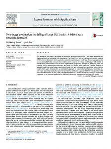
Figure 1: Multi-Layer Perceptron (left) and Radial Basis Function (right) Networks 2.2 Validation Approach
works, the latter of which form a special kind of so-called radial basis function (RBF) networks. Both kinds are universal approximators, and are widely used for pattern classification. The universal approximation property provides great flexibility and allows to model complicated decision boundaries in classification problems. Figure 1 illustrates the general layout of an MLP and an RBF network. An MLP network consists of an input layer, a series of hidden layers, and an output layer. An RBF network has a similar structure but contains only one hidden layer. The major difference between MLP and RBF networks lies in the way input is processed by neurons on the hidden layer(s) of the network. In a hidden MLP neuron, the weighted outputs of the previous layer are gathered, and a simple linear or sigmoidal shaped function is applied. In a hidden RBF neuron, however, a radial (Gauss) function is directly applied to the input vector. Such a function assumes its highest value at a centre point while continuously decreasing away from this point in all directions. The rate of decrease depends on the spread or standard deviation of the function. The closer the centre point to the input vector, the higher will be the output of the neuron. The outputs of the hidden neurons are weighted and collected at the output layer, and possibly further normalised, to obtain a final output vector. The result of using different processing functions is that, for an MLP network, pattern classification eventually comes down to drawing hyperplanes in the input space, while for an RBF network, the input space will be subdivided using hyperspheres. This subtle though important difference has great consequences for whether or not a network is suited for a particular classification task. Due to their localised nature, RBF networks are likely to be more successful when the data points belonging to one particular class are clustered in the input space. Otherwise, (too) many basis functions will be required to adequately classify the patterns.
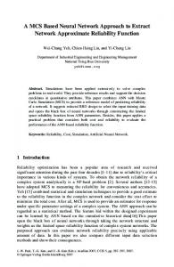
Figure 2 gives a schematic overview of our validation approach using a neural network. We assume that, as will be typical for most modelling studies, insufficient system knowledge is available to create a fully calibrated simulation model at once. Usually, a number of alternative models, or alternative model calibrations, remain open for selection. Every replication with such a model produces a training pattern for the neural network, consisting of certain behavioural statistics on the one hand (e.g., sample means and variances of time series), and of the model label on the other hand. Possibly, preprocessing of the statistics is required to reduce the information load for the network. By applying patterns from different replications across all candidate models, the network learns to identify key features of the statistics that cause a pattern to belong to a specific model. Once the network has succeeded in learning these features, data of a “replication” with the real system is offered to the network. The network output can then be interpreted as a probability vector, indicating for every simulation model the probability that the data comes from the model. The model with the highest such probability across most of the “replications” with the real system may then be retained as a valid model. 3
AN EXTENDED EXAMPLE
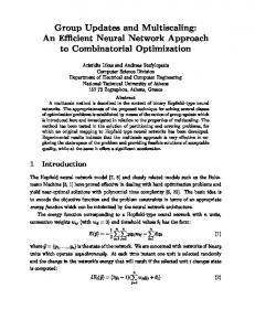
3.1 Problem Description We illustrate our neural network approach for validation on a set of simulation models for a two-class two-server queueing system with non-preemptive priority structures. The statistical properties of this system have been extensively studied by Leemans (1998). Figure 3 displays the different simulation models of interest.
906
Martens, Pauwels, and Put
Figure 2: Validation Process Overview
in Table 1. With every (ij)th element of the classification matrix corresponds the H0 hypothesis that model j is valid in light of the real system that is substituted by model i. Clearly, we expect the H0 hypothesis to be correct at diagonal entries and incorrect at off-diagonal entries of the matrix. The (ij)th element of the matrix equals the number of times that output from model i was classified as coming from model j. It gives an indication of the probability on rejecting a valid model (a type I error) for i = j and on accepting an invalid model (a type II error) for i 6= j. To give an example, the matrix in Table 1 shows that output of simulation model 1 was classified as coming from model 1 in 85% of the cases, and that in 15% of the cases, the output was incorrectly classified as coming from models 3 and 5. When simulation model 1 plays the role of the real system, there is thus a 15% chance that model 1 will be incorrectly invalidated. The probability on making a type I error when testing the H0 hypothesis at entry (1, 1) of the matrix thus equals 15%. To give another example, output of simulation models 2, 3, 4 and 5 was classified as coming from model 1 in 3.5% ( 12+2 400 ) of the cases. When the real system is substituted by any of these models, there is thus a 3.5% chance that model 1 will be incorrectly validated. The average probability on making a type II error for the
Every model consists of two servers with exponentially distributed service times. Two types of jobs arrive, class A and class B jobs, each according to a Poisson process with arrival rate 0.9. The average job service times are identical and are fixed at 1. The job type that can be handled by a server depends on the model. In model 1, class A and class B jobs are processed separately on a first-come-first-served basis. In models 2, 3 and 4, both servers process class A and class B jobs according to a non-preemptive priority rule. In particular, with regard to model 2, class A jobs have priority over class B jobs on both server 1 and server 2, meaning that no class B job will be initiated as long as there is a class A job waiting in queue. A similar statement holds for model 3. In model 4, the priority structure is heterogeneous, meaning that server 1 (2) always attempts to initiate class A (B) jobs first. Finally, in model 5, both servers take class A and class B jobs from a common queue on a first-come-first-served basis. 3.2 Classification Matrices To maximise the scope of our experiments, we treat every of the models once as being the real system, with the other models then being alternative (imperfect) simulation models. This way, the outcome of our validation method can be summarised in a classification matrix, like we showed
907
Martens, Pauwels, and Put
Figure 3: Multiserver Queueing Models
Table 1: Example Classification Matrix
the input space, we performed one set of tests using only the sample means of the queue length time series, a second set of tests using the sample means and variances of the series, a third set of tests using the sample means, variances and autocovariances for the first 2 lags, and so on, until and including autocovariances for a total of 16 lags. Thus, at the finest level of testing, 18 inputs are defined (mean + variance + 16 autocovariance lags) using 50000 queue length samples, while at the coarsest level, only 1 input is defined (mean) using 1250 samples. Since the estimated autocovariances appeared to vary substantially across the different replications, we performed a normalisation of all input data. Table 2 shows the probability on a type I error using an MLP and a PN network under the experimental set-up above. Every figure in the table coincides with the misclassification percentage of a particular classification matrix. The table also shows misclassification percentages for a well-known classification technique from statistics, i.e., the K-Nearest Neighbour (KNN) technique. This technique operates by classifying new, unseen patterns using the most frequent class label in the k-most nearby patterns; see Devijver and Kittler (1987) for details on the KNN method. We used one set of 100 replications per model to train the networks— the training set, and another set of 100 replications per model to test the networks and compute the classification matrices—the test set. Both the KNN and the PN-networkbased classification method make use of an additional set
simulation model
real system
1
2
3
4
5
1 2 3
85 0 12
0 100 0
14 0 87
0 0 0
1 0 1
4 5
0 2
0 0
3 2
92 5
5 91
H0 hypotheses at entries (2, 1), (3, 1), (4, 1) and (5, 1) of the matrix thus equals 3.5%. 3.3 Results We take the number of class A jobs in queue to be the time series of interest for validation. Two parameters are likely to influence the probability on making a type I or II error: 1) the input space for the neural networks, i.e., the number and kind of statistics that are computed from the queue length time series, and 2) the frequency at which the queue of class A jobs is sampled. As to the sampling frequency, we sampled the number of class A jobs at rates of 1/8th, 1/7th, . . . up to 5 samples per time unit. All replications were run for a total of 10000 time units. As to
908
Martens, Pauwels, and Put Table 2: Classification Errors (in %) of the KNN Method, and of PN and MLP Networks
KNN
avg PN
MLP
KNN
5 4 3
34.0 34.0 34.2
34.0 34.0 34.0
34.2 34.4 35.4
9.6 9.6 9.6
9.4 9.4 9.4
8.8 8.8 9.6
10.0 10.2 10.0
10.4 10.4 10.4
2.6 2.6 3.2
10.8 10.6 10.4
10.8 10.8 10.8
2.4 2.0 2.2
11.4 11.2 10.6
11.2 11.2 11.2
2.0 1.6 1.6
2 1 1/2
33.8 33.8 33.8
34.0 34.0 34.4
34.6 36.0 34.0
9.6 9.4 9.8
9.6 9.6 9.6
8.8 8.8 8.8
10.2 10.0 10.0
10.6 10.2 10.2
2.2 1.4 1.6
10.4 10.8 10.2
10.8 10.6 9.6
2.0 1.8 0.6
10.8 10.0 9.2
11.2 11.0 8.6
1.8 1.0 0.8
1/3 1/4 1/5
34.4 35.0 33.8
34.0 34.6 34.0
35.4 35.8 35.4
9.4 9.8 9.4
9.6 10.2 9.8
9.0 9.6 9.0
10.0 10.4 9.6
9.6 9.6 9.4
1.2 0.8 0.6
9.6 7.6 7.6
8.8 7.4 6.8
0.6 0.8 0.6
7.4 7.0 5.8
7.4 6.8 6.0
0.8 0.8 0.4
1/6 1/7 1/8
32.6 33.8 33.4
34.4 35.0 34.4
35.4 35.2 35.0
9.8 9.4 9.8
9.6 10.2 10.4
10.0 9.8 9.6
9.4 8.4 7.2
8.2 8.0 7.2
0.8 0.6 0.6
6.6 6.2 5.6
6.4 6.4 5.4
0.8 1.0 0.6
5.2 5.4 5.4
5.2 5.4 4.8
0.8 0.6 0.8
Freq
avg + var + 8 lags
avg + var PN MLP
avg + var + 2 lags KNN PN MLP
avg + var + 4 lags KNN PN MLP
avg + var + 6 lags KNN PN MLP
avg + var + 10 lags
avg + var + 12 lags
avg + var + 14 lags
avg + var + 16 lags
KNN
PN
MLP
KNN
PN
MLP
KNN
PN
MLP
KNN
PN
MLP
KNN
PN
MLP
5 4
10.8 10.6
11.2 11.2
1.8 1.6
11.0 11.2
11.4 11.2
1.8 1.8
11.0 10.8
11.8 11.6
1.8 2.0
11.6 11.6
11.8 12.0
1.8 1.2
11.4 11.6
12.0 12.2
1.0 1.4
3 2 1 1/2
10.4 11.0 10.0 7.6
11.0 11.4 10.2 7.2
2.0 1.4 0.8 0.6
10.8 11.0 9.8 7.2
11.4 11.4 9.0 6.8
1.4 1.6 0.6 0.8
10.6 11.8 9.4 6.6
11.6 11.6 8.6 6.2
1.2 1.2 0.6 0.6
11.8 11.4 9.2 5.8
11.8 11.6 7.8 5.6
1.6 0.6 0.6 0.8
11.8 11.8 7.6 5.2
11.8 11.0 7.0 4.6
1.4 0.6 0.6 0.6
1/3 1/4 1/5
7.0 5.8 5.6
6.4 5.2 4.6
0.6 0.8 0.8
6.6 5.6 5.4
6.0 4.4 4.8
0.6 0.6 0.6
5.8 5.2 5.0
4.6 4.8 4.4
0.6 0.6 0.8
5.6 5.8 5.4
4.6 5.0 4.6
0.6 0.8 0.8
5.8 5.4 6.4
5.0 4.8 5.6
0.6 0.6 0.8
1/6 1/7 1/8
4.8 5.0 5.8
4.6 5.0 5.4
0.4 0.8 0.8
5.0 5.8 5.6
4.8 4.6 5.0
0.8 0.8 0.6
5.6 6.6 7.0
5.0 5.4 5.8
0.8 0.8 0.8
6.0 7.6 8.6
5.4 6.0 7.2
0.6 1.0 0.8
7.4 8.6 9.2
6.8 7.2 7.8
1.0 1.0 1.0
of replications—the validation set—to determine optimal values for certain parameters. In the KNN method, the training set is used as a reference set to classify patterns from the validation set for an initial value of k. Classification of validation patterns is repeated for a range of values for k, and the value yielding the lowest classification error is retained. In the PN-network-based classification method, a value for the spread of the radial function of a hidden neuron must be determined. We accomplish this by first evaluating the error on the validation set for an initial family of spread values. Then, we zoom in on a selection of these values and evaluate the potential error improvement for nearby spread values. This process is terminated after three zoom levels to keep the cost of computation reasonable. The value yielding the lowest error on the validation set is retained as the final spread value. Notice here that an MLP network is trained in a different manner than a PN network. For PN networks (and the KNN method), training is designed such that no error will be made on the training set. For MLP networks, the algorithm will attempt to minimise the error on the training set, but the goal is not to achieve an error-free classifier. Instead, a technique called early stopping is used. The learning algorithm attempts to minimise the error on the training set while continuously monitoring the error on the validation set. Once the error on the validation set starts
to rise over a predetermined number of iterations, further training is believed to cause poor generalisation capabilities of the network, and the training algorithm is stopped to avoid overfitting. Classification using an MLP network produces better results than classification with a PN network, or using the KNN method. However, this goes at the expense of a much larger computation time. Classification with an MLP network took nearly 3.5 times as long as classification with a PN network and over 10 times as long as classification with the KNN method. Whereas the sampling frequency has some influence on the misclassification rate, particularly for the KNN method and PN networks at the finer levels of testing, the choice of statistics plays a much greater role. Indeed, the results significantly improve when, in addition to the mean, also the variance and a number of autocovariances are included in the input space. This is not much of a surprise as it has been shown by Leemans (1998) that some of the models have identical or at least very similar mean queue lengths for class A jobs. Adding additional autocovariance lags eventually has no effect anymore on the misclassification rate. Ideally, the mean, the variance and some of the autocovariance lags are retained in defining the input space.
909
Martens, Pauwels, and Put 4
CONCLUSION
gium. He has a master’s degree in commercial engineering of management informatics and an advanced master’s degree in artificial intelligence. His research concentrates on modelling attention in the early stages of visual processing. His email address is
[email protected].
We proposed a neural network method to validate a simulation model. We experimented with the method on five variants of a multiserver queueing model, and showed that it can be used to distinguish valid from invalid models. Our method has the advantage that multiple behavioural statistics (means, variances, etc.) can be tested simultaneously. A disadvantage of our method is that (many) replications are required with different calibrations of the simulation model to train the neural networks. In that respect, it does not allow to test individual simulation models. Further research on the subject may include an experimental study that compares our results with that of statistical techniques for validation. This study might also involve other (neural network) methods for pattern classification. The probabilistic neural network is only the simplest form of the class of radial basis function networks, and it is possible that other variants perform better. Finally, the relation between the probabilities on making a type I and II error are worthwhile to investigate.
FERDI PUT is professor at the Department of Applied Economics of the Catholic University of Leuven, Belgium. He teaches numerous courses, including Data Communication and Computer Networks, and Simulation Theory and Applications. His e-mail address is
[email protected].
REFERENCES Balci, O. 1998. Verification, validation and testing. J. Banks, ed. Handbook of Simulation. Wiley, New York. 335-393. Bishop, C.M. 1995. Neural Networks for Pattern Recognition. Oxford University Press, Oxford. Devijver, P.A., and J. Kittler. 1987. Pattern Recognition: Theory and Applications. Springer Verlag, Berlin. Kasabov, N.K. 1996. Foundations of Neural Networks, Fuzzy Systems, and Knowledge Engineering. MIT Press, Cambridge, MA. Leemans, H. 1998. The two-class two-server queueing model with non-preemptive heterogeneous priority structures. Department of Applied Economics. PhD thesis, Katholieke Universiteit Leuven, Belgium. Nauck, D., F. Klawonn, and R. Kruse. 1997. Neuro-Fuzzy Systems. Wiley, Chichester. Wasserman, P.D. 1993. Advanced Methods in Neural Computing. Van Nostrand Reinhold, New York. AUTHOR BIOGRAPHIES JURGEN MARTENS has a Ph.D. in Applied Economics from the Catholic University of Leuven, Belgium. His research interests include discrete-event simulation, data mining and operations research. He carries out various projects for the Belgian airline industry. His e-mail address is hjurgen
[email protected]. KARL PAUWELS is a Ph.D. student at the Neurophysiology Laboratory of the Catholic University of Leuven, Bel-
910