A neural network architecture for learning temporal ...

A neural network architecture for learning temporal information Adriaan G. Tijsseling & Luc Berthouze Cognitive Neuroinformatics Group, Neuroscience Research Institute, AIST, Tsukuba Central 2,Umezono 1-1-1, Tsukuba 305-8568, JAPAN phone: +81-298-615369 fax +81-298-615841 [email protected]

1

A neural network architecture for learning temporal information Abstract In this paper, we propose a neural network architecture that is capable of the continuous learning of multiple, possibly overlapping, arbitrary input sequences relatively quickly, autonomously and online. The architecture has been constructed according to design principles derived from neuroscience and from existing work on recurrent network models. The network utilizes sigmoid-pulse generating spiking neurons to extract timing information from the input stream and it modifies weights using an adaptive learning rule with synaptic noise. Combined with coincidence detection and an internal feedback mechanism we have a learning process that is driven by dynamic adjustment of the learning rate. This gives the network the ability to not only adjust incorrectly recalled parts of a sequence but also to reinforce and stabilize the recall of previously acquired sequences. The performance of the network was tested with a set of overlapping sequences from a toy problem domain in order to analyze the relative contribution from each design principle. Keywords: temporal information, recurrent neural network, autonomous Hebbian learning, sequential learning.

1

Introduction Sequential information is at the heart of any cognitive activity. Picking up and throwing a

ball, deriving mathematical formulas, reading text, driving a car, using a vending machine: Any cognitive system has to deal with sequential information embedded in perception and action. To create such a system, we therefore require an artificial neural network that is capable of learning and recalling temporal series of sensory stimuli, internal states, and action responses. Several neural network architectures and algorithms have been developed to address the problem of sequential learning, each one applied to a specific problem domain. Modifications of backpropagation have been suggested to handle various sequence generation and prediction tasks. Well-known examples are Jordan (1986) and Elman (1990) networks.

2

Since the backpropagation method employs supervised learning, applications of these networks are restricted to those domains where teaching signals are readily available. Recently, Hochreiter & Schmidhuber (1997) have enhanced recurrent backpropagation to shorten the time it takes to learn a sequence and to solve reported problems with error signals backpropagating through time. Wang & Arbib (1993) describe a possible short-term memory model based on unsupervised learning, one that uses a population of neurons in which each neuron locally codes a single item of a sequence. A neuron may have multiple terminals that are deployed as follows. The first terminal stores the state of the most recent input to the element, the second terminal stores the second most recent external input to the element, and so forth. With this method, sequences up to a length K, possibly containing ambiguities, can be recalled. The requirement is that the length K does not exceed the capacity of the network as indicated by the number of its neurons. This may become a shortcoming of this model when dealing with multiple sequences. Dominey (1995) shows how a sensory-motor sequence learning model with leaky integrator neurons is able to learn to associate four sequences, built from the same 5 elements, but in permuted order, with 4 different action responses. The model consists of two components, the first of which generates unique activation patterns to represent the current state of a sequence. These patterns are associated with a correct response by the second component. As such, learning a sequence is reduced to an interplay between staterepresentation and associative memory. Unfortunately, while the model does not suffer from capacity problems, it does have difficulty with complex sequences, i.e. in which an element can have more than one successor, as in p 0→p1→p0→p2→p0→p1→p0→p3 (Dominey, 1995; Jones & McLaren, 2001).

3

Each of the above models solves one or more problems with sequence learning (prediction, generation, recognition (Sun & Giles, 2001)) when applied to one or more simple or complex sequences. Although they have their benefits, our motivation is to provide a temporal sequence learning network that can perform autonomously, continuously, and on-line. It should detect and learn new regular patterns of sensorimotor interaction so that it can either predict or reproduce them whenever it is placed in similar conditions, and it should do so without any external regulation. Patterns should be recalled in their original order and with preserved timing information, and, upon cueing, can complete sequences when presented with a pattern from any position in the particular sequence. Naturally, these networks should also be tolerant to certain amounts of noise in the input. A property we found lacking in the above models is that there appears to be no internal method to determine whether the network is actually recalling the learned sequence and not producing a random recall. The experimenter is, of course, able to verify a correct recall by observing various performance indicators (level of activation, weight configuration, etc.), but these kinds of information are not directly available to the model itself. In other words, is there a way to have a network verify if its recall, given a certain trigger input, matches a previously acquired sequence? What happens when the network is stimulated with random patterns? Perhaps it will recollect a sequence that has nothing to do with what was learned. It is, after all, possible that the generated outputs are the result of straying in memory space by natural trajectories of instability. The network presented in this paper has been developed to support such a mechanism using coincidence detection and internal feedback loops (which essentially makes information on internal states available as input to the system itself). It also addresses other considerations we found relevant for autonomous learning of sensorimotor sequences, such as the role of context, catastrophic interference (French, 1994), synaptic noise, and an adaptive learning rate

4

using a local learning rule. We will elaborate upon each in turn, illustrating how these considerations become design principles for possible sequence-learning network architectures. After introducing the network, we proceed with an analysis of its performance with single random sequences as well as a set of overlapping sequences from a real problem domain.

2

Design principles of the network Designing a neural network architecture requires applying design principles that constrain

its structure and function. We base these constraints on the idea that the richness of human cognitive behavior is in some way related to the neuropsychological structure and function of human information processing, providing us with possible design principles to guide the construction of a neural architecture. The following sections describe each one in turn. 2.1

The role of context

Learning a sensorimotor sequence always occurs in context. Following Wallenstein, Eichenbaum & Hasselmo (1998), we use the term “context” to refer to a stimulus environment that is changing much more slowly than the specific stimuli being learned. The context not only contains many meaningful regularities, it also generates invariants due to its stability over time (Chun & Jiang, 1998). On a related note, Gibson (1966) suggested that the perceptual system adjusts itself to invariant information from the environment. As such, context provides a structured environment, which can be exploited to coordinate behavior (Reber, 1989). Any analysis of novelty and familiarity requires the concept of context, since all understandable novelty exists within a relatively stable context that is not novel (Baars, 1988; Gray, 1995). The relevance of context in storage and recall of sequential information has been studied thoroughly. Within the animal domain, the role of spatial context cues in the recall of

5

visuomotor associative memories in honeybees has been experimentally demonstrated (Collet et al., 1997). With respect to humans, it was found that the error made by 7-12 month old infants in Piaget’s classic A-not-B task (Piaget, 1954) was highly sensitive to context (Smith et al., 1999). For example, the error was not made when the two containers A and B are made visually distinct. Theories of hippocampal functioning also stress the role of context (Hirsh, 1974), based on ample evidence that suggests that the hippocampus is necessary for the formation of normal associations between focal stimulus events and the context in which they occur (Eichenbaum, Otto & Cohen, 1994). Levy and Wu (1996) argued that encoded context is required for both learning and storage of context as well as sequence prediction in a hippocampal system. Based on experimental studies, impairments of phonological working memory may cause lack of learning ability of phoneme sequences in Broca’s aphasics, because ambiguous sequences containing higher-order sequential dependencies can only be learnt when preceding sequence events are maintained temporarily in some kind of context memory (Goschke et al., 2001). An interesting illustration of the role of context is found in a study of motor learning. It is suggested that context triggers appropriate motor responses (Brindley, 1969). A question raised was whether one can train body parts to a specific task, without the adaptation spilling over to other tasks performed by the same body parts. When a subject’s arm is trained on overhand throws and then tested on underhand throws, for most individuals the overhand training does not carry over to the subsequent underhand throws (Thach, Goodkin & Keating, 1992). Yet, the overhand training persists through to subsequent overhand throws, readapting with repeated throws. Thach (1996) compared this to using a similar movement that is differently calibrated for two different contexts, for example, hitting a baseball with a bat versus hitting a tennis ball with a racquet. Modifying the activity of baseball hitting does not

6

affect the activity of the tennis game. However, if the two movements become more similar, in the case of playing squash and tennis, carry-over is more likely to occur. Given these considerations we have assigned context a substantial role in our to be described network. Contextual cues can help the network in learning to separate two similar sequences. To maintain a sequence in memory while processing a new one, however, requires resolving the stability-plasticity dilemma. 2.2

Adaptive learning rate and the plasticity-stability dilemma

How can a learning system be designed to remain plastic, or adaptive, in response to significant events and yet remain stable in response to irrelevant events? Plasticity is necessary for the incorporation of new information in a network. Stability means keeping previously acquired knowledge intact. A solution to this trade-off is to find a mechanism that is able to distinguish between old and new and to use this information to control the learning process. The architectural properties of a neural network place strong constraints on what can and cannot be learned (Grossberg, 1982, 1987; Karmiloff-Smith, 1992; Tani & Nolfi, 1997), exhibiting a trade-off between a flexible architecture and the stability of stored knowledge. Structurally unconstrained networks may suffer serious performance problems when they assume total interconnectivity between all nodes (e.g. Hopfield, 1982) or a hierarchical, multilayered structure in which each node in a layer is connected to all nodes in the layers just above and below it (e.g. Rumelhart, Hinton & Williams, 1986). Backpropagation networks, for example, are highly plastic in that they can, in principle, learn any input/output mapping and, as such, any detectable feature of the input set (Funahashi, 1989; Hornik, Stinchcombe & White, 1990). Too much plasticity, however, often leads to catastrophic interference, which is mainly evident during pure sequential learning (French, 1991, 1994; McCloskey & Cohen, 1989): If the network is trained on one set of input-output relations and is then presented with a new set of input-output relations that is different from the previous set, the weight matrix

7

may change substantially, with the effect that prior representations are partly or completely forgotten. In other words, the minima of the objective function for one training set may be totally different than the minima for subsequent training sets. Suggested solutions to the stability-plasticity dilemma are commonly based on modularity and localist information processing (Carpenter & Grossberg, 1988; McClelland, McNaughton & O’Reilly, 1995; Murre, Phaf & Wolters, 1992). To avoid possible potential for catastrophic interference in our network, we adopt a novelty-based learning rate, based on ideas in ART (Carpenter & Grossberg, 1988) and CALM networks (Murre, Phaf & Wolters, 1992). Novelty-based learning implements a known psychological distinction between elaboration and activation learning (Graf & Mandler, 1984). The former type of learning results in the formation of new associations while the latter type merely strengthens existing associations. The magnitude of the rate of learning is determined by two other processes in the network, coincidence detection and internal feedback, both of which determine the relative novelty of presented information. 2.3

Coincidence detection

In the context of our network, coincidence detection means that the network has the ability to detect if a particular sequence has been encountered previously in the continuous stream of incoming information. The mechanism of coincidence detection that we use is inspired by temporal and spatial integration of information in biological dendrites (Stuart & Häusser, 2001). Temporal integration of signals in dendrites is realized by amplification of backpropagating action potentials through oscillations. This amplification is sensitive to the relative timing of action potentials with the phase of oscillations. Additionally, spatial integration is caused by local effects on action potential amplitude restricted to the site of synaptic input. In sum, coincidence detection provides a mechanism that links the global activity of a neuron with the activity of specific sets of inputs, providing a key function to

8

associative learning (Stuart & Häusser, 2001). In our case, we will show it implements novelty-based regulation of learning by actively linking the learning rate to the novelty of a sequence. Apart from dendritic coincidence detection, we employ another neurobiological finding, synaptic noise, as design principle. 2.4

Synaptic noise

The concept of synaptic noise is of relatively recent interest in the field of neurobiology. According to White, Rubinstein & Kay (2000), noise in the nervous system might have a number of roles. It might constrain the coding accuracy in neural structures (Zador, 1998); enhance signal detection under some circumstances (Collins et al., 1995); or affect the firing patterns of multimodal sensory neurons (Braun et al., 1997). Moreover, Anderson et al. (2000) showed how noise contributes to the contrast invariance of orientation tuning in the visual cortex of cats, since it allows for the averaged membrane potential of a neuron to be translated into spiking in a smooth and graded manner across a wide range of potentials. With respect to recurrent neural networks, applying synaptic noise to the learning process has been shown to improve convergence time and generalization performance to longer sequences (Jim, Giles & Horne, 1994). Consequently, adding synaptic noise to the weight adaptation in our network might not only be beneficial for overall performance, it may also provide insights into the possible functions of biological noise. The remainder of this paper is outlined as follows. First, we will describe our network for learning multiple sequences in detail and examine the role of the various parts of the network in its performance. Subsequently, the performance with a problem domain containing multiple, overlapping sequences is then tested and analyzed. This is followed up with a conclusion and a discussion on categorization with this sequence learning network.

9

3

Technical description of the sequence learning network architecture

3.1

General overview of the network

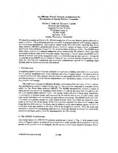
Figure 1 shows the schematic of a candidate network architecture for learning sequential information, which we will refer to as “SequenceNet” in the remainder of this paper. The network is organized in modular fashion with each module performing a specific function in the overall learning process. The input module, output module, coincidence detection module, and each layer in the central module all have the same number of neurons. The size of the context module is equal to the size of the predicted context module, but this size may differ from the size of the other modules. The basic idea is as follows: Information is presented in sequential fashion to the input module, which – in the scope of this paper – is just a placeholder. Contextual information, on the other hand, is fed into the context module, the size of which is arbitrary, and it represents either information about the relatively slowly changing environment in which the sequence occurs or any information arriving from other sensory modalities and brain areas (e.g. linguistic information or an associated memory). Activation is then propagated to the central module, which contains a set of layers with leaky integrator neurons (described in section 3.2). The input module has fixed one-to-one connections with 1.0 weights to each layer (i.e. values are just copied), while the context module has fixed all-to-all connections with random weights. Each central module layer itself is connected in an all-to-all fashion with both the output and the predicted context modules, connections that contain the only modifiable weights in the network. There are no connections between central module layers. The output of the output module is propagated to a coincidence detection module via fixed weights (see section 3.4 for details). This component employs a mechanism that discovers regularities in the stream of activation passing through the network and uses this data to regulate the rate of learning in the network.

10

coincidence detector

output

predicted context

central layers

input

context

α

coincidence detector

w00 w01 w02 w03

w0n

output

Figure 1. The left panel shows the schematic of the architecture of the neural network for learning sequential information. The input layer is a placeholder for each pattern in a presented sequence, while the context layer receives both external contextual information as well as feedback information from the predicted context module (i.e. the context that the network has learned to associate with the current sequence). Input and context information as well as feedback from the output module is propagated to the central module that contains a variant of spiking neurons. This module is responsible for extracting the variety in timing information from the input. All learning occurs in the connections from the central module to the output and the predicted context modules. The output module is also connected to the coincidence detector module, which regulates the learning rate by calculating the familiarity of the current output based on a history of previous states.

The function of the network is to learn or predict the next pattern in a sequence, such as for example p1→p2→p3→p4. Suppose that at time t, pattern p1 is presented as input. The output

11

module should learn to associate the next pattern p2 at time t + 1 with p1 or, if it has already learned the sequence, reproduce p2. An efferent copy of the output of the network at time t + 1 is sent back to the central module. Berthouze (2000b) shows this will not only enable the network to learn the spatio-temporal nature of presented stimulus sequences, but that it could also be used to train the network to generate a sequence. In other words, the activities of the output layer can be trained to mimic the next stimulus entering the input layer (Hopfield, 1982; Kleinfeld, 1986). Apart from generating the next pattern in a given sequence, the network also learns to predict the context that is associated with the sequence. This will provide the network with the capacity to restore sequences in cases where context cues are only partially available, for example, when the sequence in question is part of a task that has to be applied in a new environment (Tani & Nolfi, 1999). The central module plays a crucial role in the extraction of timing information from the activation of the input, output, and context modules. This incoming activation is integrated using a function described in section 3.5. Each layer in the central module has a different time constant and each layer will consequently process the incoming activation differently. The actual learning process then takes place in the connections – which are the only modifiable weights – between both the stored context and output module and the central module. After pattern p1 has been processed by the central module, the weights are modified using the activations from the central module and information about the next pattern, p2, which is now present in the input module. In the following sections we will describe each module in detail. 3.2 3.2.1

Leaky integrators with continuous output pulses Spike Accumulation

The design of the neurons in the central module is based on the Spike Accumulation Model by Shigematsu, Ichikawa & Matsumoto (1996). Each SAM neuron has an accumulated potential that is calculated using leaky integration of incoming input spikes:

12

(1)

ui (t ) = ai (t ) + τ ⋅ vi (t −1)

in which, for SAM neuron i and at time t, ui(t) is the accumulated potential, vi(t) is the internal

€

potential, ai(t) is the incoming input activation, and τ is the decay rate of the internal potential vi(t). The internal potential is defined with respect to accumulated potential and the neuron’s output (which, in the original SAM cell, is defined by a Heavyside applied to the accumulated potential) as: (2)

v i ( t ) = ui ( t ) − ρ ⋅ oi ( t )

in which ρ is the subtraction constant of the internal potential.

€

3.2.2

Time constants

The parameters τ, ρ and T are crucial for determining the time constant of the SAM neuron. In biological systems, neurons can be in one of three states: Quiescent, excited or refractory states (Milton, Mundel & van der Heiden, 1995). When the voltage ui exceeds the threshold T, neuron i fires, changing its state from quiescent to excited. Immediately after firing, the neuron becomes refractory, during which it cannot be excited (the absolute refractory period, which lasts about 1 to 3 ms) or with much difficulty, i.e. a higher input (the relative refractory period, which lasts about 5 to 200 ms). The relative refractory period is the direct result of an interplay between two factors: First, the rapid decay of the threshold to its resting value (which is complete within 3-5 ms) and, second, the slower decay of the membrane hyper-polarization to its resting potential (complete within 60-200 ms). In the SAM neuron, this relative refractory period is controlled by the ρ parameter, the subtraction constant of the internal potential after the generation of an output spike. The absolute refractory period, on the other hand, is not controlled by any parameter, but is in this paper fixed “de facto” by the duration of one computing cycle (alternatively, one could introduce a time delay in the computation, such that the network only receives inputs between large intervals, e.g. at times t, t + 3, t + 6, …). Given these parameters 13

τ, ρ and T, one can adjust the refractory period such that the generated spike stream varies in onset and/or in duration and, hence, how much of the previous incoming activations the SAM neuron will accumulate. Consequently, we define the time constant of a SAM neuron as the combination of the onset and duration of the generated spike stream. With respect to the function of the SAM neuron as a building block in a model of temporal sequence processing, the main point of interest is the memory capacity of a SAM neuron. Berthouze (2000b) shows how these factors together can be empirically chosen to select a particular time-constant. Given a single incoming spike at some time t, the factors we can then use to describe a SAM neuron’s memory capacity are the time elapsed until the neuron emits a pulse, the duration of this pulse, and the amount of time it takes the neuron to settle back into quiescent state. Consequently, the time constant of a SAM neuron will determine the network’s processing capacity of sequential information. If we have several layers of SAM neurons, each layer implementing a different time constant, then we have a network that is able to encode the timing information contained in a presented sequence. 3.2.3

Sigmoid output pulses

Since SAM cells are spiking neurons, the output activity is defined as a series of discrete events. Spiking neurons can be relevant at the neural level, but since our network should be considered at a more abstract level, we are concerned with an averaged activity of neurons. Several researchers have studied the dynamics of neural systems using averages of the mass activity of large numbers of neurons (Freeman, 1975; Gerstner, 1998). The effect of averaging is to smear the all-or-nothing threshold potential of individual neurons into a sigmoid relationship between local mean dendritic potential and local mean firing rate (Robinson, Rennie & Wright, 1997). Such a mean firing rate could then be approached using sigmoid functions and would contribute to the generalization behavior of the network (Tsuda & Kuroda, 2001). For this reason, based on the accumulated potential, the modified SAM

14

neuron is subjected to a sigmoid function that introduces continuity, but preserves the idea of a “pulse”-like response:

(

oi ( t ) = f ( ui ( t )) = 1 1+ e

−c ( ui ( t )−T )

)

(3)

in which c is the efficacy constant of the accumulated potential ui(t) and T is the firing €

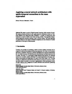
threshold. Aspects of the nonlinear function for pulse generation are shown in figure 2. The threshold moves the sigmoid function along the horizontal axis, raising or lowering the minimum activation needed to contribute to the accumulation of input spikes. The c parameter modifies the shape of the sigmoid. The higher c is, the more similar the function will be to a plain binary threshold function. In biological systems, this form of nonlinearity is also present in dendritic trees. Dendrites are said to be compartmentalized due to neuron-specific differences in morphology (Häusser, Spruston & Stuart, 2000; Mel, 1993) with each of these dendritic compartments applying expansive nonlinearity to boost synaptic input (Mel, 2000). c = 20, T = 0.9 c = 8, T = 0.6 1.0

0.5

0.5

1.0

Figure 2. Possible sigmoid output pulses of a modified SAM neuron, for c = 20 and T = 0.9.

Nonlinear output pulses generate a more stable performance in the network with respect to perturbations in the input sequence. We found that sigmoid pulses do not require a unique, empirically determined set of parameters to find a solution to a given problem domain. Instead, the system will learn a particular sequence with a wider range of parameters, offering an additional aspect of robustness (Tijsseling & Berthouze, 2001). In a similar way, sigmoid

15

output pulses have been employed in order to constrict the number of possibly confusing solutions in the selection of foveating points in a moving sequence of images (Watanabe et al., 1999). 3.3

Weight modification

The output of all modified SAM neurons in the central module are sent via all-to-all connections to both the output module and the context module. Since the learning process is identical for both output and context module, we focus on the former in describing the learning process. The neurons in the output module perform population coding on the combined activities of the modified SAM neurons from each layer in the central module. The activation of an output neuron i is updated according to: H

I

ai = ∑ ∑ w ijk ⋅ o kj

(4)

k= 0 j= 0

in which k runs over the number H of layers in the central module and j runs over the number €

I of neurons in layer k (note that this number equals the number of neurons in the input and output module). This rule will produce the following output for a given output neuron i: oi = 1 (1+ e−a i )

(5)

The weights from each layer k in the central module to the output layer are updated €

according to an error-correction rule with synaptic noise. We define this as follows for a given layer k: (6)

Δw ij = α ⋅ (in i − out i ) ⋅ o j + η

in which ini is the activation value of neuron i from the input module (the activations of which

€

represent the next pattern in the sequence), outi(t) is the output of neuron i from the output module, o j(t) is the output of modified SAM neuron j, α is the learning rate, and noise

16

parameter η is a random value in the uniformly distributed range of [–η min, ηmax]. This learning rule forces the weights to adapt to the difference between the actual output and the feedback information from the input module, multiplied by the activation distribution in the intermediate layer. Note that at the time of weight modification, the input module holds the next pattern in the sequence. This means that the weights are modified such as to minimize the difference between the output and the next pattern in the sequence, because the intended role for the output module is to predict the consequence of the current pattern. 3.4

Coincidence detection module

The coincidence detection module’s role is to detect if a particular sequence has been encountered previously in the continuous stream of incoming information and to use this information to regulate the learning rate α. This gives the network the ability to only modify weights if a given sequence is novel and to resort to base-rate learning with familiar sequences. The neurons in the coincidence detection module are each tuned to a unique time constant δ, meaning that they can only process activations at certain time intervals t, t + δ, t + 2δ, and so on. These neurons also retain a history of previous input signals, necessary for comparison with the current input signal. These input signals arrive from the output module over connections that have fixed weights – configured as in the bottom panel of Figure 1 – such that each weight increases in strength with each connection to a given coincidence detector neuron. For example, the weights from each output module neuron to the first coincidence detector neuron may have the connection strengths 1.0, 2.0, 3.0, 4.0, n ⋅ 1.0, respectively. This implementation mimics spatial dendritic compartmental integration that makes it possible to distinguish between sequences that are spatially different, but which have a similar or equal signal strength (Mel, 2000; Stuart & Häusser, 2001). By using various time delays and differently weighted connections, the output from the coincidence layer will be the result of both spatial and temporal integration.

17

In a biological dendritic neuron, many inputs may be received constantly. The extent of dendritic spread allows significant spatial integration, whereas the integrated membrane potential at the neuron body varies slowly in potential, allowing inputs that occur at different time frames to integrate. The formal implementation is as follows. The input ai of each coincidence detector neuron i is calculated as: N

ai (t ) = ∑ w ji ⋅ oOj

(7)

j

In which oOj is the output of connected output neuron j, N is the number of output neurons, €

and wji is the strength of the connection from output neuron j to coincidence detector neuron i. € output of the coincidence detector, oCD , is then calculated using its history of retained The i

input activations:

€ 1.0 if a(t ) − a(t − δ ) < T CD o (t ) =  0.0 else

(8)

CD

In which TCD is the threshold and δ is the time constant of the coincidence detector neuron. €

This activation rule implements the idea that a coincidence detector neuron will fire only if its state matches the stored state from the time t - δ. The threshold covers the cases when there is a certain amount of degradation or noise in the input, making it possible for the neuron to fire, even if the states do not closely match. The function of the coincidence detector layer is to actively modulate the learning rate of the network. When one or more coincidence detector neurons fire, because the current state matches a previous state, the learning rate should consequently be lowered. With no neurons firing, the learning rate should increase so that learning of the new sequence is facilitated. Formally:

18

α (t −1) + λ + λ ⋅ β ⋅ ε if ∑ oCD ≥ 1 i  i Δα (t ) =  α (t −1) − λ − λ ⋅ β ⋅ ε else

(9)

In which λ is a constant denoting the amount of change in the learning rate α ; β is a €

momentum term to accelerate learning rate change if it is in the same direction as the previous update as indicated by ε: 1.0 if ∑ oCD (t ) ≥ 1.0 and∑ oCD (t −1) ≥ 1.0 i i  i i  ε = 1.0 if ∑ oiCD (t ) < 1.0 and∑ oiCD (t −1) < 1.0  i i 0.0 else 

(10)

The change in learning rate should, however, not increase linearly as we want suppressed €

learning with familiar inputs and quick adaptation to novel inputs, i.e. only learn when learning is necessary, while base-rate learning will make it possible for the network to further stabilize its learned sequences in the absence of novel inputs with very small weight changes. A solution is to subject the learning rate change to a bounded sigmoidal function:   , if (α (t ) + Δα ) < 0.0 b  α ( t ) = b + α max , if (α (t ) + Δα ) > α max  (11) max  b + α max −  α , otherwise with :  f ( x)   1+ e  f ( x ) = (c y α max )Δα − c x

(12)

€

max in which α is the maximum value for the learning rate and b is the base-rate value. The

€

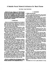
sigmoid is fitted within the range of 0.0 and α max using the constants cx and cy, as shown in figure 3. cy defines the slope of the sigmoid, while cx shifts the sigmoid along the x-axis. This function allows for asymptotic approach to either base rate or maximum learning rate, while allowing for a fast change in learning rate in the intermediate cases (i.e. when a sequence is

19

becoming familiar). In other words, if a new sequence is presented only once, the learning rate will be affected marginally, yet, if it is presented again, the learning rate will increase stronger. 0.1

0.05

0.05

0.1

Figure 3. Nonlinear learning rate function in which the maximum learning rate is set to 0.1 and cx and c y set to 7.0 and 12.0, respectively.

The above implementation of coincidence detection can be interpreted as a functional equivalent of local dendritic coincidence detection, described by (Stuart & Häusser, 2001) and discussed in section 2.3. The key features to this mechanism are adapted as follows. The activations from the output module need to match the coincidence detector neuron's activations from its history of previous states. In dendrites, more synaptic inputs need to cooperate before the dendrite becomes active. In the model, coincidence detection increases its effect with each matching pattern in a sequence, producing a positive response. Furthermore, the above implementation also produces a local effect on action potential amplitude, restricted to the site of synaptic input, by the differently weighted connections between the output and the coincidence detector module. The latter contributes to spatial integration of input signals. The coincidence detection process in our network and the dendritic coincidence detection effectively share the property that they link the global activity of a neuron with the activity of specific sets of inputs. According to (Stuart & Häusser, 2001), this provides a key function to associative learning.

20

1.5

Activation propagation to the central module

As mentioned in section 3.1, each of the modified SAM neurons in the central module receives activations from the input, output, and context modules. The input module is – within the scope of this paper – just a placeholder for a given pattern in a sequence. The context module, on the other hand, produces an output that is a merge of external contextual information with activations from the predicted context module. This allows for reconstructing a sequence’s correlated context if the external contextual input has been degraded due to noise. Modified SAM neurons in the central module, in turn, receive a combination of the activations propagated from the input and context modules, as well as the output module. Feeding output activations back into the network is not novel. For an example of this approach see Jordan (1986), in which the activation propagated to the hidden layer is the sum of input and context, divided by 2. In our network, the activation propagated to a modified SAM neuron, for a given index i and central module layer H, is calculated according to the following input function: H

a =

o I − oO ⋅ o I + oO + oC

(13)

2.0 + o I − oO

in which aH is the activation propagated to the ith modified SAM neuron in layer H, and

€

neurons oI, oO, and o C are the output values of the ith neuron from, respectively, the input, output, and context modules. The value 2.0 in the denominator ensures that the activation to the central module remains within the range [0.0, 1.0] (please recall that connections between output and central and between input and central module are one-to-one connections with fixed weights of strength 1.0). For neurons in the input module, the output value is identical to the input value. The context module, on the other hand, is fully connected with the central

21

module with fixed, uniformly distributed, random weights, wC, from the range [-1.0, 1.0]1. For the context module, oC is then calculated as follows:

  oCi = f  ∑ w Cji aCj   j 

(14)

with f a simple sigmoid function:

€

f ( x ) = 1.0 (1.0 + e−x )

(15)

and aC the activation of a neuron j in the context module. This activation is updated using €

external information and activations from the stored context module via one-to-one connections. C

a =

i C − o PC ⋅ i C + o PC

(16)

1.0 + i C − o PC

in which oPC is the output of the stored context module and iC is the input from external

€

contextual information. Given this activation function, the network can execute a sequence even when the external contextual information degrades or is subjected to noise, since it is able to rely on internally recalled contexts. The activation propagation function defined by equation 13 provides additional support for novelty learning in combination with the coincidence detection module described in the previous section. When a sequence is old, the difference between oI and o O approaches zero and the network will resort to stabilization, because the next input will match the current output, realizing an automatic recall of the current sequence. The learning rate will be low and, as such, memory of learned sequences will only be reinforced. On the other hand, when a sequence is new, the learning rate, modulated by the coincidence detection mechanism, increases until the sequence has been stored in memory. The efferent copy from the output

1

We opted for random weights, but a fixed set of values is also possible. If the context layer size is identical to the size of the hidden layers, one could instead use a one-to-one mapping of context to hidden layers. 22

module, therefore, not only functions as internal feedback, but also to automatically detect previously acquired patterns. Equation 13 only applies to binary-valued inputs as it allows for output-regulated propagation of activation. When the input is zero, the propagated activation becomes

(o

O

+ c ) (2.0 + oO ) and when the input is at maximum value, this becomes

(1.0 + c ) €

(3.0 − o ) . In both cases, the network has to perform a two-fold task of reducing oO O

to zero or increasing it to maximum, respectively. For real-valued inputs, this propagation

€

function breaks down as input values are not restricted to two binary values, forcing the network to learn an unnecessary complex nonlinear input-output mapping. Instead, the following propagation function is used (Jordan, 1986): aH =

o I + oC 2.0

(17)

We will show that this novelty-based procedure of propagating activation to the central €

module prevents overtraining and reduces catastrophic interference by providing a solution to the stability-plasticity dilemma. Learning multiple sequences in this context-driven dynamic learning network will not cause catastrophic interference with previously stored information, but instead the network will conduct stabilization processes to maintain the integrity of all acquired sequences.

4

Simulation details

4.1

Training procedure

The task of the proposed network is to learn sequential information quickly and online, so that learned sequences can be completed when the network is cued with either a possibly incomplete pattern or possibly partial contextual information. The general procedure is to train the network on a sequence plus its associated context (the context is always the same for

23

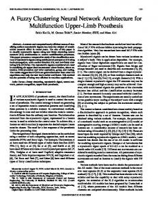
all patterns in a given sequence) until the learning rate has dropped to base-rate learning or until the number of epochs has reached a predefined upper limit. After successful training, the network is then tested on its recall of the acquired sequence. This occurs by initially presenting the first pattern of the sequence (although we also test on recalls from other positions in a sequence) plus its context and then let the network update its internal states for a given number of iterations. This means that the output of the network becomes its next input. An additional consideration with training procedures concerns the possibility of non-cyclic sequences. Since the SequenceNet is essentially a recurrent network, one would naturally apply it to infinite length or cyclic sequences. As described in section 3.3, the network updates its weights based on the difference between the output and the next input, the latter of which functions as a teaching signal. When the end of a sequence is reached, the next stimulus can be of several possibilities. In the case of cyclic sequences, the next input becomes the first pattern of the sequence again, but what if a sensorimotor sequence is supposed to terminate when finished? To this extent, we will also verify the ability of the network to recognize when a sequence needs to be terminated. Two possibilities are explored: In the first one, we set the next stimulus for the last pattern to be a vector with low-amplitude, uniformly distributed noise in the range of [0, 0.05]. In the second one, it was set to the last pattern of the sequence itself. In a recall phase, cyclic sequences show up as periodic orbits. Figure 4-A illustrates a sample orbit for a sequence A→B→C→D→E (see section 4.2.2), produced during a recall that lasted for 100 time steps. The orbit is defined by the triple

∑ a ( t − 2),∑ a ( t − 1),∑ a ( t) i

i

i

,

which corresponds to the sum of activation of all nodes i in the central module at three subsequent time-steps. There are five distinct basins of attractions in the network,

24

corresponding to the five patterns of sequence A→B→C→D→E. When pattern E has been trained with A as a teaching signal, the activation propagation passes through each pattern in the sequence, and returns to state A if the last pattern E is reached. The orbits corresponding to recalls of terminating sequences are shown in figures 4-B and 4-C. Training with a noise signal as an indicator of the end of a sequence creates a large attractor basin for this terminator, whereas using the last pattern as a terminator produces a recall that ends in a small orbit centering on pattern E. These three kinds of sequences will be employed in a later section that reports the performance of the network when learning multiple sequences.

Figure 4: Activation flow over time during recall of sequence A→B→C→D→E. In panel A, the final pattern ‘E’ is trained on the first pattern ‘A’. In panel B, the final pattern is trained on a vector of low-amplitude noise. In panel C, the last pattern is trained on itself (Note that in panel C, the cube is rotated 90 degrees counterclockwise for better viewing purposes).

Regarding multiple sequences, the training procedure is modified to allow for a balanced learning of all sequences such that the possibility of interference is reduced. Initially, the network is trained with the first instance from a permuted set of sequences plus the corresponding context for 10 iterations or until the learning rate has dropped to base-rate learning (this constitutes one single epoch). After training, the network is tested on the recall of the sequence. If the recall is correct, the network is trained on the next sequence (this constitutes one single block). If recall is incorrect, the current sequence is retrained (i.e. one more epoch is added). After a new sequence has been added, both sequences are retrained until each one is recalled correctly. Only then does training proceed further (i.e. one more block is completed). An epoch is therefore defined as a single training of the current subset of

25

sequences, and a block as the complete successful training of this subset of sequences. The simulation ends when all sequences are recalled correctly or when the number of epochs exceeds a predefined criterion. In the latter case, the network is said to have failed the learning task. This training schedule is also used by Dominey (1995). The necessity of retraining all sequences is to prevent instabilities that emerge when training a subsequent sequence shifts or “tips” the weights too much. In other words, the network finds a local minimum that solves the current sequence, but not all sequences. Repeatedly training all sequences forces the network to search for a global minimum. Dominey (1995) manually changes learning rates for complex sequences to prevent deadlocks in the system. In our case, this is not necessary as we use an internally regulated dynamic learning rate. The additional benefit of this dynamic learning rate is that there is no need for an external observer to regulate the learning of multiple sequences. In other words, since the system settles to consolidation with a previously acquired sequence, the learning rate drops to base-rate learning and there is no risk of overtraining a sequence such that weights shifts become too large. The procedure of learning a new sequence only after successfully acquiring a previous sequence can be related to human skill learning. Josephson & Hauser (1981) describe how in learning to play table tennis, the player moves to a higher level only if at the current level few negative reinforcements occur. If performance at a given level is poor, the player may achieve proper skills at a lower level first. Such stage-like acquisition of skills is a central concept in Piaget’s theory on development of sensory-motor skills (1954) and it is also observed in higher-level cognitive processes such as problem-solving skills. For example, Carlson et al. (1990) provide experimental data that shows that practice leads to strategic restructuring of cognitive processes at several levels of organization.

26

4.2

Training sets and parameters

Two different training-sets were used for the simulations in section 5. We either supplied the network with random single sequences or a set of sequences from a given problem domain. The following two sections describe each training-set in turn and the accompanying parameter values for the network. 4.2.1

Random sequences

When training the network with single sequences, we used sequences that consist of binary patterns constructed by means of a random distribution. The binary values of these patterns were picked in such a way that for each bit the value was set to 0 if a generated random value was below 0.3, and 1 otherwise2. Using these random sequences we tested the effect of sequence length, pattern size, the number of layers in the central module, or the amplitude of noise, and experimentally determined the scope and limits on duration of learning, recall performance, and memory storage capacity. For all simulations using single sequences, we set the context to zero inputs. In other words, the context is not used in single sequence simulations. For all simulations, we applied the same set of parameters as to show the robustness of the system. These parameter values are specified in Appendix I, unless explicitly mentioned otherwise. The decay rate and subtraction constant were distributed over each layer in the central module, starting at the maximum value listed in the referred table and reduced linearly in steps of “maximum value” / (“number of layers” + 1). Additionally, for each coincidence detector neuron we incremented the time constant δ with 5.0, but the initial time constant varied with the length of a sequence so that the coincidence detector module is able to detect repetitions. Naturally, it would be preferable to use random values for the time constants, but to restrict the number of free variables, we have chosen for this linear increase in time

27

constant. Likewise, the connection weights from the output layer to each coincidence detector neuron were incremented with 1.0, starting from an initial 1.0 value. The momentum term and threshold in the coincidence detection module were set, respectively, to 0.0 and 0.025, such that the learning rate would not decrease too quickly. 4.2.2

Multiple, overlapping, and branching sequences

In simulations that test the performance with overlapping and branching sequences, we employed a training set from a suitable existing problem domain. These sequences were derived from the Playstation™ game “Tekken™” by Namco™. In this game, fighting characters can be controlled by a human player using a console. In particular, one of the available characters can be controlled to perform a connected sequence of wrestling moves. Given two distinct single moves (starters), which we define as A and F, the human player has to memorize the next possible move to combine each single move into a sequence. Figure 5 shows the so-called multithrow chart that describes the possible strings starting from A and F. A

B

C

D

E

J

F

G

D

E

J

H

K

I

K

E

J

K

Figure 5. Multi-throw chart for the character “King” of Namco™’s “Tekken™” Playstation™ game, obtained from an internet published move-list documentation. Each letter indicates a single move, which can only be connected with the move associated with the linked letter to create a wrestle sequence. Sequences can only start with either of the two moves A and F (see text for details).

2

Thresholds of 0.5 and 0.7 have also been used, but the network simulation results with patterns from these three values showed low variance, and we have therefore only used the results from a threshold of 0.3. 28

For example, given starter A, the player has to press a set of buttons to execute move B, after which he or she has the option to stop or to execute either C or G, and so on. There are 10 possible complete sequences, 6 starting from starter A, and 4 from starter F. Learning all sequences requires many training trials, and usually the game-player will not be able to produce a complex sequence based on a starter, but instead produce a shorter sequence (personal observation). We converted each move into a 16-bit vector, corresponding to the direction the character has to move to (which occurs only in the starter move), and each of the 4 possible buttons that have to be pressed (see Appendix II for button and move details). The context for each sequence is also a 16-bit string, indicating for each sequence its starter and its index (details in Appendix II). All layer sizes were set to 16, with the central module containing 8 layers. For all simulations, we again applied the same set of parameters as to show the robustness of the system (Appendix I). For each coincidence detector neuron we incremented the time constant

δ with 1.0, starting from a value of 5.0. The connection weights from the output layer to each coincidence detector neuron were also incremented with 1.0, starting from 1.0. The momentum term and threshold in the coincidence detection module were set, respectively, to 0.25 and 0.10, in order to have learning settle quickly into base-rate learning, such that weights are not shifted too strongly between training different sequences. For each of the three sequence types described above 25 simulations were done. These types are coined as follows: “cyclic” refers to sequences in which the last pattern is followed by the first pattern; “end” and “noise” refer to both terminating sequences where the last pattern is followed by, respectively, itself or a noise signal. Sequences were presented either in permuted order or in linear order (top down order of Figure 5) according to the training schedule described in section 2.6. The maximum number of epochs was set to 5000. If a simulation failed to learn within this criterion, it was restarted.

29

We looked at the following factors: Can the network be trained to recall a sequence that terminates in the last pattern as opposed to a recall in which the last pattern loops back to the first one? What is the capacity of the network in acquiring sequences? Is there a “preferable” sequence, in the sense that some sequences may be easier to recall than others are? How are sequences learned? Is the network able to separate single moves from the entire sequence or does it represent sequences as wholes? We will address these questions using qualitative analysis of the experimental data, although quantitative details are discussed elsewhere (Berthouze & Tijsseling, 2003).

5

Simulations

5.1

Introduction

We describe a series of simulations that illustrate the performance of the network in learning sequential information and the effect of the various network components. The simulations are grouped in three sections: They are simulations that present (1) the performance of the architecture, (2) the learning behavior with multiple sequences, and (3) the justification of the design principles. For the first group we also provide a comparison with an Elman (1990) network to elucidate the various improvements the proposed network offers. We chose the Elman network because it is a widely used recurrent network for sequential learning. A detailed description of an Elman network can be found in Elman (1990). In short, an Elman network is a three-layered feed-forward neural network that uses the backpropagationthrough-time learning method (Williams & Peng, 1990). The unique feature of this network is that it contains an extra, so-called context layer that stores a copy of the previous hidden layer activation values which are then presented as part of the input activation of the network. These feedback connections allow the network to process past state information, a

30

requirement for sequential learning. Learning proceeds similar to the SequenceNet: An input is presented and the network has to learn to map the output to the next input, which therefore acts as a teaching signal. To access past state information, a copy of the hidden unit activations is stored in the context layer and fed back into the hidden layer in the next activation update. Because the Elman network only has access to the state of previous time step and is trained with the interference-prone backpropagation method (French, 1991; McCloskey & Cohen, 1989), we predicted that the Elman network would have difficulty with sequences that contain a variety of timing information, such as repeated patterns. The next section describes simulations testing the performance of the proposed network and comparisons with an Elman network. 5.2 5.2.1

performance of the architecture Effect of sequence length

We varied sequence length from an initial 5 patterns to a maximum of 75 patterns, in steps of 5. For each sequence length, 10 different random pattern sets were created and both the SequenceNet and the Elman network were trained on each sequence for 10 different runs. The SequenceNet had 8 layers in the central module and the size of all layers was set to 16, equal to the pattern size. The Elman network had a hidden layer with the size set to 16 in order to approximate the SequenceNet central module layer size. Figure 6 shows the average number of epochs required to train a given sequence, displayed in a logarithmic scale. The correlation between the number of epochs and the length of a sequence is exponential for both networks, but the Elman network required on average 33 times more epochs and failed to learn sequences that are longer than 25 patterns within the pre-set limit of 100,000 epochs, whereas the SequenceNet managed to learn up to a length of 60. The range in epochs, indicated by the error bars, also increases with sequence length, but

31

this is most likely an artifact of using random patterns, since a longer sequence length means adding more degrees of freedom in the dimensionality of the patterns. Effect of sequence length on learning

epochs

100,000

10,000

1,000

100 SequenceNet ElmanNet 10 5

10

15

20

25

30

35

40

45

50

55

60

length of sequence

Figure 6. Effect of sequence length on learning for both the SequenceNet and the Elman network. The horizontal axis displays the length of the trained sequence, and for each length, the vertical axis shows the required number of epochs (in logarithmic scale).

5.2.2

Effect of number of central module layers

The selection of number of layers in the central module in the previous simulation was not chosen arbitrarily, but instead was derived from exploring the effect of the number of layers on the network’s recall performance. In this simulation, the number of central module layers varies from 1 to 50 and the network had to learn a random pattern sequence of length 10. A similar simulation with an Elman network was also executed, but in which the number of hidden units were varied instead. Since the role of the hidden layer in Elman is different from that in the SequenceNet, this comparison only serves an illustrative purpose. Figure 7a displays the error in recall for the SequenceNet for a task that required learning a random pattern sequence of length 10, but with the number of layers varying from 1 to 50. The recall error sharply decreases initially until a maximum recall performance is reached. With each extra layer, however, the performance can become instable, with some networks 3

Thresholds of 0.5 and 0.7 have also been used, but the network simulation results with patterns from these three

32

failing to learn the sequence. These are classic cases of underlearning and overlearning. Overlearning occurs with fewer than 7 layers, in which the weight space has become too small to reliably store the sequence. With too many layers, a situation of underlearning occurs where the network not only finds the global minimum for the learning task but also ends up in local minima, out of which it cannot escape with the noisy weight adaptation, since the number of degrees of freedom in the system has become too large. 0.50

recall error

0.45

0.40

0.35

0.30

0.25

0.20

0.15

0.10

0.05

0.00 1

3

5

7

9

11

13

15

17

19

21

23

25

27

29

31

33

35

37

39

41

43

45

47

49

number of layers mean squared error

average number of epochs

MSE

MSE

6

5

10,000 9,000 8,000 7,000

4

6,000

3

5,000 4,000

2

3,000 2,000

1

1,000

0

0

2

3

4

5

6

7

8

9

10

11

12

13

14

15

16

2 4 6 8 10 12 14 16 18 20 22 24 26 28 30 32 34 36 38 40 42 44 46 48 50

number of hidden units

number of hidden units

values showed low variance, and we have therefore only used the results from a threshold of 0.3. 33

Figure 7. The top panel shows the effect of the number of central module layers on the recall performance of the SequenceNet. Recall performance is measured using a summed square of errors between the recalled sequence and the correct one, averaged over the number of patterns in the sequence. The bottom panels display the corresponding simulation for the Elman network, using hidden layer size as a variable and measuring performance with mean squared error and average number of epochs. The Elman network learns successful if the number of hidden units is larger than 8. It does not suffer negative effects from an oversize hidden layer.

The results for the Elman network are vastly different. A minimum mean squared error criterion of 0.01 was not reached after a maximum of 50,000 epochs for a hidden layer with fewer than 9 nodes (Figure 7b). For 9 nodes and more, the number of epochs needed to reach criterion approaches a minimum value of 1000 epochs asymptotically (Figure 7c). There were no negative effects in using very large hidden layer sizes (up to 100), which is a known aspect of backpropagation networks (O’Reilly, 2001). With the SequenceNet, adding extra layers to the central module will provide the network with more resources to encode the presented sequence, as long as possible pitfalls for underlearning are avoided. With each additional layer, a different time constant arises, and a new dimension is created in the weight space from central to output module. Yet, the performance remains dependent on the random nature of the sequence. Due to randomness, the degrees of freedom over patterns – which can be visualized with a histogram – fluctuate, with lesser degrees of freedom meaning longer training times. Another factor is the occurrence of subsequences or repeated patterns. These factors can be easily illustrated with a small sequence. We used ten different sequences of length 5 and pattern size 4. The number of epochs required for correct recall for each of these sequences ranged from 932 to 30797, depending on the sequence. This variation in epochs can be correlated to the spread of the histogram of the activities of the patterns in a sequence as well as the distance between each adjacent successive pattern of a sequence (i.e. between p1 and p2, p2 and p3, etc). Figure 8 illustrates this correlation. The number of epochs shows an inverse correlation with distance (measured with 3 different Minkowski distance

34

functions) as well as spread of the histogram, although the correlation is weaker in the latter case . correlation of epochs and sequence complexity

distance

9 8

supremum

7

euclidean

manhattan spread

6 5 4 3 2 1 0 0

5000

10000

15000

20000

25000

30000

epochs

Figure 8. The number of epochs required to train a sequence is correlated with the complexity of this sequence, as approximated by the distance between successive patterns (using Minkowski functions) or a histogram of the spread of activities of patterns in the sequence.

5.2.3

Effect of pattern size

Using sequence lengths in the range of 5 to 50, we next tested the effect of pattern size on learning performance. In the previous simulations, the size of random patterns in a sequence was set to 16. Figure 9a and b reveals the effect of pattern size on the required number of epochs for successful recall with the SequenceNet and the Elman network, respectively. Pattern sizes varied from 4 to 20 in steps of 2. For each size, a graph of the logarithmic number of epochs for each sequence length is shown, averaged over 10 sequences and 10 runs. By reducing pattern size, the distances between successive patterns will become shorter and, given the analysis from Figure 8, we indeed observe increases in the required number of epochs.

35

effect of pattern size on epochs (SequenceNet) 100,000

epochs (logarithmic)

10,000

1,000

4 6 8

100

10 12 14 16 18 20

10 5

10

15

20

25

30

35

40

45

50

pattern size

effect of pattern size on epochs (ElmanNet) 100,000

epochs (logarithmic)

10,000

4

1,000

6 8 10 12 14 16 18 20

100 5

10

15

20

25

30

35

40

45

50

pattern size

Figure 9. For each pattern size along the horizontal axis, the vertical axis displays the number of epochs that was required to train the corresponding sequence (in logarithmic scale). The top panel shows the data for the SequenceNet and the bottom panel for the Elman network. The performance of the SequenceNet not only reveals faster learning but also the ability to learn longer sequences, compared to the Elman network.

As with the simulations testing the effect of sequence length, the learning performance of the Elman network is several degrees of magnitude slower than that of the SequenceNet. In

36

addition, the Elman network fails to learn sequences longer than 35 patterns. The difficulty the Elman network has in acquiring long sequences can be attributed to the fact that its architecture only allows for capturing a single time constant, i.e. the state from the previous time-step. The SequenceNet, on the other hand, employs several modified SAM cell layers with each tuned to a different time constant. As such, it can capture more aspects from the presented sequence of information. This observation becomes evident in the next simulation. 5.2.4

Encoding of timing information

A necessary feature for sequence learning is that the network is able to encode timing information. So far, the simulations concerned sequences such as p0→p1→…→pn, but the performance of the network needs to be verified for sequences where individual patterns or subsequences are repeated, such as p0→p0→p0→p1→p1→…→pn. Given a sequence of length 5 and pattern size 16, we trained the network on increased sequence complexity (which we define here, for simplicity, as the length of a sequence given a fixed order of 5 elements, A, B, C, D, and E), starting from a lowest complexity A→B→C→D→E (no repetitions, length 5), and incremental repetitions: A→A→B→C→D→ E (length 6), A→ A→B→B→C→D→E (length 7), and so forth. The final sequence trained had length 26 and composed as (omitting arrows) AAAAAABBBBBCCCCCDDDDDEEEEE. For longer sequences, the number of epochs required for successful recall exceeded a preset criterion of 20,000 for 3 of the 5 sequences. Figure 10 shows the logarithmic number of epochs required to train a given sequence, averaged over 5 repetitions of 5 different random pattern sequences of a given complexity. Error bars indicate the range in epochs. Similar to the data from learning various sequence lengths, the network shows robust and fast learning, but with an exponential increase as timing information becomes more complex, an observation that indicates the limits of the capacity of the network for the given task. The Elman network, on the other hand, failed to

37

learn any sequence that had at least one repetition, as was expected given the results of the previous simulation. Encoding of timing information

100000

epochs (logarithmic)

10000

1000

100

10 5

6

7

8

9 10 11 12 13 14 15 16 17 18 19 20 21 22 23 24 25 26 timing length

Figure 10. The effect of complexity of timing information on the required number of epochs to train the corresponding sequence. Epochs are displayed in logarithmic scale to produce a clear difference between range of epochs for each timing complexity.

We also tested the SequenceNet on repetitive subsequences. We chose the sequence ABCDABCEABCFABCGABCH from Dominey (1995), which is characterized by the repetitive subsequence ABC followed with a different patterns D, E, F, G, or H. This sequence was learned after an average of 1322 epochs, producing a correct recall when cued with the first pattern A. When the dynamic learning rate adjustment was turned off, this sequence could not be learned by the network. Learning complex timing information as contained in this sequence requires fine-tuning of weights, which can only be assured by a dynamic learning rate. This allows for low weight changes in the event of a familiar pattern so that the network’s weight configuration does not get warped and correct recall will be disrupted. 5.2.5

Effects of noise in recall cues

Robustness to noisy input was investigated by training the network with a sequence of 16 orthonormal patterns from 〈1,0…,0〉 to 〈0,…,0,1〉 and cueing a recall with any of these 38

patterns. These cues, however, were distorted by adding uniformly distributed noise in the range of [–x,x]. Figure 11 shows for each value x from 0.2 to 0.4 (including 0.5 and 1.0) the average error in recall over points in a sequence and over 10 different noise distributions. An error below 0.08 corresponds to correct recalls from any point in the sequence. An error above 0.8 indicates not one single correct recall has been made. Not surprisingly, the recall error is maximal with a noise distribution between –0.5 and 0.5. However, increasing the range of noise to [–1,1] will in some cases lead to correct recalls. These cases comprise of noise values that distort a pattern to such extent that it becomes similar to another pattern in the learned sequence. Recall with random noise

1.0 0.9 0.8

recall error

0.7 0.6 0.5 0.4 0.3 0.2 0.1 0.0 0.20

0.22

0.24

0.26

0.28

0.30

0.32

0.34

0.36

0.38

0.40

0.50

1.00

amount of noise

Figure 11. Recall error for noisy input. The error is the average error over points in the sequence and over ten repetitions. The error bars denote minimum and maximum error.

5.3 5.3.1

learning behavior with multiple sequences Performance for the Tekken sequences

The left-hand panel of Figure 12 shows the average number of epochs that was required to train all sequences of Figure 5 for each type of sequence (one cyclic and two with terminators) and in permuted order. This average number increased with the addition of each new sequence. At the same time, the number of iterations required to train each sequence until

39

the learning rate has dropped to base-rate learning decreased (right-hand panel of Figure 12). This suggests that once the structure of the input domain is known, the network is merely fine-tuning weights in order to generate correct recalls for all sequences. permuted sequence presentation

epochs

550 500 450

cyclic

400

noise

350

end

300 250 200 150 100 50 0 1

2

3

4

5

6

7

8

9 blocks

10

average number of iterations per block

iterations

10

9

cyclic noise end

8

7

6

5

4 1

2

3

4

5

6

7

8

9 blocks

10

Figure 12. The top panel displays the average number of epochs over 25 successful runs for each sequence type, with sequences presented in permuted order. The bottom panel shows the average number of iterations required to train each sequence. The maximum number of epochs was set to 5000.

The number of epochs it took to train a set of sequences was found to be dependent on the overlap between the new sequence and the previously acquired ones. This became evident when sequences were presented in the order as they appear in Figure 5, the results of which

40

are shown in Figure 13. Each new ‘A’-sequence required an increasing number of epochs, in particular the last 2 ‘A’-sequences, which not only share a long partial sequence, but also introduce a new branch at move ‘G’. The large overlap between these two sequences became evident when the last two ‘F’-sequences were introduced. These not only share the first 4 moves with each other, but also the same ‘G’ branch with the previously mentioned ‘A’sequences. The required number of epochs to train the whole set after adding the last two ‘F’sequences was relatively larger. linear sequence presentation

epochs

550 500 450

cyclic

400

noise end

350 300 250 200 150 100 50 0 1

2

3

4

5

6

7

8

9 blocks

10

Figure 13. Average number of epochs for sequences presented in linear (successive) order.

Additionally, a sudden stronger increase in epochs may occur, which corresponds with the entire weight space being reconfigured in order to accommodate a new sequence such that each learned sequence is correctly recalled given a cue and an associated predicted context. This occurred when presenting the 7th “end”-sequence, which is the first ‘F’-sequence. A closer look at a sample simulation provided additional evidence for weight rearrangement when introducing sequences. Figure 14 shows the changes in range and variance of the weights from central module to output module after presenting the 2nd, 4th, 5th, and 10th sequence. The number of epochs required to learn the 2nd sequence was 6 and the

41

corresponding weight changes were low in amplitude. Learning the 4th sequence required only 3 epochs, and the variance was low, indicating that memory for this sequence fitted well into the existing weight configuration. Adding the 5th and 10th sequence required far more epochs (15, resp. 48) with an increased variance in weight changes; and for the last sequence, an exponential increase in the range of weight changes was observed. range

7.0

variance

0.30

6.5 6.0

0.25

5.5 5.0

0.20

4.5 4.0

0.15

3.5 3.0 2.5

0.10

2.0 1.5

0.05

1.0 0.5

0.00

0.0 2

4

5

2

10

4

5

10

Figure 14. Range (left panel) and variance (right panel) of weight changes after adding sequences 2, 4, 5, or 10.

5.3.2

Differences between sequence types

Although the overall learning performance was qualitatively similar for each type of sequence, there were quantitative differences between cyclic sequences and terminating sequences, evident from the overall slower learning with terminating sequences. In particular, “end”-sequences showed sharply degraded learning after 6 blocks. For 5 of 25 permutations of the sequence-set the network failed to learn all “end”-sequences within the required amount of epochs, mastering only up to 7 to 9 sequences. Although the network was able to learn all “noise”-sequences, it also had increasing difficulty with incorporating each new “noise”-sequence. These capacity problems are suggestive of Miller’s well-known 7 ± 2 limitation of short-term memory (Miller, 1956). A probable cause for the differences in learning difficulty for the three sequence types lies in the effects of the presence of a terminator. When the terminator is a noise signal, the network learns, in fact, an extra category. This category contains all the various noise signals and, as shown in figure 4B, the corresponding attractor basin may become quite large. A

42

similar explanation can be made for sequences terminating in the last pattern itself. Figure 4C showed that terminator patterns (e.g. E) develop wider category boundaries than nonterminator patterns (e.g. C). We verified this possibility by training only one single “end”sequence, A→B→C→D→E, and observing the developing recall performance of the network while it is acquiring this sequence. After 10 iterations, the network recalled the sequence4 A→EΟ. With each additional iteration, the recalled sequence improved gradually from A→B→EΟ to A→B→C→EΟ to A→B→C→D→EΟ, but still remained instable. This can be seen in Figure 12, where training the first “end”-sequence required about 8 times as many epochs compared to the other two sequences, although it only needed far fewer iterations for each epoch. These extra epochs were needed to stabilize the recall of the terminating sequence, because the pattern E attractor was relatively strong. For “noise”-sequences, the noise category was not relatively stronger. It only became an extra category to be learned. 5.3.3

Structure of sequence representations

An interesting question to ask is what the structure of the network’s acquired sequential representation is. Specifically, are sequences represented as a whole, or does the network recognize the single patterns that compose a sequence? As a rough approximate of the network’s representation of the sequence structure, we analyzed the total activation value over time of all central module units during the recall of each sequence. If the network is representing single patterns as well as entire sequences, then the total activation for a single pattern can be assumed to be at the same level, irrespective of the sequence it is part of. If the learning process is based on entire sequences, then there should be no relation between the total activation of the recall of a single pattern for each sequence. Since recalls of each

4

We will use arrows between moves in a sequence when there is potential confusion between cyclic and terminating sequences. A looping arrow at the end of a sequence means that the last move is being recalled infinitely. 43

sequence proved to be stable orbits, the total activation of the recall of a single pattern over time is of roughly the same value.

total activation

IE IJK B-IJK

IJK

A-GH-E B-DJK

H-K

DJ

B-DJK

I-K

H-E G-K

DJ

DJK

DJK

I-E

A-GH-K B-IE

C-K

DJK

G-K

A-GD-K

DE DE

DE

A-CD A-CD

G-E

DE ABCDE ABCDJK

B-DE

ABGDE

G-E

B-DE

ABGDJK ABGHIE ABGHIJK

C-E

A

B

C

D

E

G

H

I

J

K

moves

Figure 15: Total activation levels for each pattern during recall of respective sequences. The horizontal axis displays the possible patterns cq. “moves”, from Figure 5 and the vertical axis displays the total activation of each particular pattern during recall in each of the sequences it is part of. For example, “A-CD” refers to those sequences containing pattern ‘A’ and ending in the subsequence “C→D”.

Figure 15 shows the total activation values for each pattern and sequence containing starter ‘A’, obtained from a single simulation with cyclic sequences. It can be observed that total activation values vary strongly based on the sequence a given pattern is part of. Hence, we cannot claim that patterns are represented separately from the sequence they are part of. It does, however, not imply directly that representations are based on entire sequences only. There is evidence that the total activation level of a single pattern is related to the patterns that

44

precede or follow it, i.e. on the timing information of a given sequence. We can relate the different activation levels of a given pattern by verifying the other patterns that are shared by the sequences it is part of. For example, pattern ‘A’ in sequence A→B→C→D→E has an activation level close to that of sequence A→B→C→D→J→K. Activation levels for pattern ‘A’ in sequences containing ‘G’ are higher, and can be further distinguished by the terminator that is shared by their respective sequences. Sequences ending in ‘K’ are more similar in activation level compared with sequences ending in ‘E’. The same observation can be made for other patterns in the chart. Activation levels increase when a given pattern is preceded or followed by one or more different patterns. This suggests that the network is able to correlate between partial sequences and, based on this, create a similarity structure for the sequences it has acquired. Consequently, predictions about the learning performance of new sequences can be made. For example, a new sequence that conflicts with the network’s acquired similarity structure will require relatively more epochs before it can be recalled correctly. This will be explored in the next section. 5.3.4

Exploring the similarity structure by explicitly training subsequences

We showed that the SequenceNet appears to create a similarity structure from the training set based on overlapping parts. To test this observation, we used an alternative training method. We not only presented the sequences from Figure 5, but also their subsequences, such as, for example, A→B, A→B→C, A→B→C→D. This lead to a total number of 21 sequences in Figure 5. Using this method, we create a richer similarity structure by introducing extra overlapping sequences. Would this increase the learning difficulty of the network because a given pattern may now be followed by more alternative patterns? For example, G could mark the end of a sequence, be followed by D, by D→E, or by D→J, and so forth. Alternatively, would it make it easier because it implicitly suggests a clustering method? For example, training A→B→C→D→E and A→B→C→D→J→K may require less

45

training if the network applies similarity between partial sequences using an earlier acquired A→B→C→D sequence. We also tested the effect of adding a new sequence. We argued in the previous section that a prediction could be made about the network’s learning performance when presented with a new sequence. If this sequence does not match the similarities learned by the network, it should require relatively more epochs to learn. Three different kinds of a new sequence were created: One containing a new starter L, one ending in a new move M, or one connecting previously unlinked moves (i.e. which introduces a shortcut). We focused our analysis on linear sequence presentation (starting from A→B and ending with F→G→H→I→J→K) to avoid any performance differences based on variances in the order of sequence presentation. Figure 16 displays, for 25 different simulations and each sequence type, the average number of epochs required to train all 21 sequences. Since the presentation of sequences was successive, the labels for the horizontal axis display the latest sequence that has been added. Over the first 13 learning blocks – containing only ‘A’-sequences –, learning progressed similarly for the three sequence types, showing near equal epoch levels. After that, learning performance varied. Contrary to the previous simulations with the 10 complete sequences, networks trained on “noise”-sequences performed similar to those trained on cyclic sequences. “End”-sequences, on the other hand, required many more epochs during training. With “noise”-sequences, there still is only one extra category for noise signals, but in the case of “end”-sequences, all patterns, except the starters and moves E and K, become both terminator as well as non-terminating pattern. Since terminator attractors can become relatively strong attractors, learning to differentiate between B as a non-terminating move and B as a terminator consequently required more training epochs.

46

linear sequence presentation

epochs

400

350

cyclic end noise

300

250

200

150

100

50

FGHIJK

FGHIE

FGHI

FGH

FGDJK

FGDE

FGD

FG

ABGHIJK

ABGHIE

ABGHI

ABGH

ABGDJK

ABGDE

ABGD

ABG

ABCDJK

ABCDE

ABCD

ABC

AB

0

blocks

Figure 16. Average number of epochs over 25 simulations required by the network to learn the 21 sequences from Figure 5 (subsequences as well as complete sequences). The entire set of sequences was presented in linear order.

The training procedure was such that a set of sequences was repeatedly trained until each one of them was recalled correctly. By verifying which sequences needed retraining after presenting a new sequence, it was possible to observe whether a new sequence required rearrangement of the network weights or whether it could be easily recalled after a few training iterations. The stacked line chart in Figure 17 displays the trend of the contribution of each “noise”-sequence to the total number of epochs over all blocks. For example, the collected data showed that adding sequence A→B→C→D→E only required an average of 4 epochs before the current set of sequences was correctly recalled, during which A→B was never retrained, A→B→C 25% of the average total epochs, A→ B→C→ D 50%, and A→B→C→D→E 100%. Once the previous sequences were acquired, adding

47

A→B→C→D→E only required training this new sequence and reinforcing the previous additions, which meant that the network was mainly learning to link E with D. Adding A→B→C→D→J, on the other hand, required more training: Previously, a recall trajectory passing D would end in E, if the context indicated this sequence. With the new addition, the network also had to learn to separate D→ J and D→J→ K from D→ E subsequences. This observation is persistent over training blocks: Adding sequence A→B→G required retraining of all sequences that include the subsequence A→B→ C, since it introduced an alternative branch at move ‘B’. The only sequence not being retrained was A→B. 600

500

400

300

200

100

FGHIJK

FGHIE

FGHI

FGH

FGDJK

FGDE

FGD

FG

ABGHIJK

ABGHIE

ABGHI

ABGH

ABGDJK

ABGDE

ABGD

ABG

ABCDJK

ABCDE

ABCD

ABC

AB

0

Figure 17. Stacked line chart of the percentile contribution of each sequence to the number of epochs required to train a current set of sequences, starting with sequence A→B, which is the first sequence presented to the network. The horizontal axis displays the most recent sequence added and the corresponding line in the graph shows its contribution to the number of epochs.

Further addition of sequences with alternative endings repeatedly necessitated minor retraining of overlapping sequences. When a new pattern was introduced, as with “H” in A→B→G→H, additional epochs were required to incorporate the new pattern as well as the extra subsequence G→ H. In addition, A→ B required more training trials with the introduction of a new starter “F” in sequence F→G. The above observations indicate that the

48

learning of sequences proceeds by extracting the underlying similarity structure, defined by overlapping parts and branching parts. What would happen if we added a new starter or a new move, or if we created a new sequence based on existing patterns? We trained the network on the 21 “noise”-sequences, and then presented one of 6 new sequences. For each new sequence, the same weight configuration was used from training the previous 21 sequences. This was done to eliminate variances in epochs due to variations in weights. The 6 new sequences were grouped in 3. A→B→G→H→M and F→G→H→M tested the addition of a single new terminator. F→C and L→C tested connecting two moves that have not been used in the same sequence. To verify the effect of adding F→C on previously acquired ‘F’-sequences, we also linked a new starter ‘L’ to ‘C’. Finally, we tested creating a shortcut between two previously indirectly connected moves using sequence F→H and compared this with L→H, which introduces a new starter ‘L’. Figure 18 shows the number of epochs, averaged over 10 simulations that were needed to train the final set of sequences after adding one of the 6 new sequences. "noise"-sequences 2500

2000

1500

1000

500

0 abgm

fghm

fh

lh

fc

lc

Figure 18. Differences between average number of epochs required to train one of 6 different possible new sequences. The black line shows the standard deviation.

49

Introducing a new terminator ‘M’ did not have a significant effect on the required number of epochs to train the final set of sequences. A→B→G→H→M was trained comparatively faster, but that may have been the result of ‘A’-sequences being trained more often over all blocks (The linear presentation starts with ‘A’-sequences). Strong differences appeared when comparing the training of F→H with L→ H. The former sequence required nearly 1500 epochs more than the latter. Figure 19 shows the percentage of maximum epochs required to train all ‘F’ sequences after adding F→H, compared to adding L→H. F→H creates a novel branch from starter F, forcing the network to retrain F→G and F→G→H, and in a lesser extent other sequences containing G→ H, in order to accommodate the new possible trajectory. It is possible that the network is unable to learn “shortcuts” (as F→H is a shortcut of F→G→H). However, training the network on just these three sequences did not show any performance and learning problems. Training “shortcuts” may still be harder than training

% of epochs

“normal” sequences, as can be observed when comparing F→C and L→C. 100 90

fh

80

lh

70 60 50 40 30 20 10

new

FGHIJK

FGHIE

FGHI

FGH

FGDJK

FGDE

FGD

FG

0

Figure 19. Percentage of epochs required to retrain a sequence after the addition of a new sequence, F→H or L→H.

50

5.4

Justification of the design principles

5.4.1

Role of noisy weight adaptation

The effect of using noise in the adaptation of weights is shown in Figure 20. We trained the network on a random pattern sequence of length 10 and size 16, using noisy signals in the range [-x, x] in which x was varied from 0.0000001 to 0.001.The bold horizontal line at y = 714 denotes the number of epochs needed to train the network in absence of noise. When x exceeds 0.001, the number of epochs increases exponentially, since the network is not able to fine-tune the weights for a given solution anymore. The large noise values create too large shifts in weight sets. The optimal range of noise in this situation appears to be for x between 0.00034 and 0.00044. Effect of noise

738

epochs

728

718

708

8.9E-04

9.3E-04

8.6E-04

7.9E-04

8.2E-04

7.5E-04

7.2E-04

6.8E-04

6.5E-04

5.8E-04

6.1E-04

5.4E-04

4.7E-04

5.1E-04

4.4E-04

4.0E-04

3.7E-04

3.3E-04

3.0E-04

2.3E-04

2.6E-04

1.9E-04

1.6E-04

1.2E-04

8.8E-05

5.3E-05

1.8E-05

2.9E-06

1.5E-06

1.0E-07

698

noise

Figure 20. Adding noise to the adaptation of weights leads to overall faster convergence of training. With too large noise values over 0.001, this effect disappears and learning becomes intractable.

51

Overall, the advantage of noisy weight adaptation is that, indicated by a lower number of epochs, the network is able to find a solution at a quicker pace. It may also be the case that using noise, possible local minima can be escaped. If the learning process of the network is visualized as a ball rolling over an energy surface, adding noise to the weights may push this ball out of a shallow curve and into a deeper one. These advantages of noise are sensitive to the range of random distribution used to generate the noisy signals. 5.4.2

Effect of context on learning

In the introduction, we discussed the role of context in sequence learning and how it provides a slower changing stimulus environment to which the network can adjust itself. We furthermore claimed that any analysis of novelty and familiarity requires the concept of context, since all understandable novelty exists within a relatively stable context that is not novel (Baars, 1988; Gray, 1995). To test the relevance of context on multiple sequence learning, we ran a simulation using cyclic sequences, but without supplying contextual information. The network failed to learn a second sequence; it was not able to recall both sequences correctly, displaying a clear catastrophic interference effect (French, 1994). This interference was caused by repeated shifts in the weights during the learning of each sequence. The first presentation of a sequence required a rounded average of 20 epochs in order to get a correct recall. After this initial learning period, switching between sequences required an additional rounded average of 3 epochs before recall of the current sequence was correct. In fact, we found that the weight configuration before and after presenting a sequence showed a small unidirectional shift. The correlation between these two sets of weights showed to be significant (> 0.9).

52

0.10 0.08 0.06 0.04 0.02 0.00 -0.02 -0.04 -0.06 -0.08 -0.10

0.0008

0.0006

0.0004

0.0002

0.0000

-0.0002

-0.0004

Figure 21. Changes in weights over time during training of two sequences without context information. The bottom panel zooms in on the last part of the top panel.

Figure 21 shows the changes in weight of the efferent connections from a single neuron in the central module to the output layer during the course of learning. Starting from an initial uniform zero weight (left panel), the changes are large in magnitude, then decrease and finally settle into a low amplitude oscillatory regime (right panel), switching between a configuration that solves the first sequence to one that solves the second sequence. Since there is no information separating the sequences, the recall performance of the network is one that can turn to either sequence when cued with the first move ‘A’. 53

5.4.3

Recalls with partial context cues

The effect of the feedback loop from the predicted context module to the context module provides the network with the ability to reconstruct the context in the event the input context contains noise or is distorted. If we sever this feedback loop, however, additional information on the representation of sequences acquired by the network can be obtained by looking at the trajectory during recalls with partial contexts. In previous simulations, each context specifies the starter and the index of the sequence to be trained or recalled. To verify recall trajectories with partial context cues, we provided only the starter of the sequence. We hypothesized that the network will show a recall that reflects an orbit passing parts of the easiest reproducible sequences. When the network had been trained on “end” sequences, cueing a recall with only 'A' and a context indicating the starter, the recalled sequence is B→EΟ. As discussed earlier, training “end” sequences leads to relatively strong attractors corresponding to the terminators of each sequence, such as e.g. ‘E’ and ‘K’. This recall with a partial context cue provides additional evidence for such strong terminator attractors. With ‘F’ as a starter, however, the “end” sequence recalled is a single pattern GΟ. But since pattern ‘G’ is core to eight different sequences, this recall showed that the network lacked the necessary additional information to produce a full sequence, terminating its recall on ‘G’ itself. Early termination due to insufficient information was shown by setting the context to zero. This lead to a recall that switched between B and G, both of which are the two subsequent patterns of, respectively, starters ‘A’ and ‘F’. Recalls with partial context information for networks trained with “noise” sequences showed a different picture compared to “end” sequences, as there was no relatively stronger terminator attractor present. With a context denoting starter ‘A’, the recall repeatedly showed either sequence B→C→ D or, less frequently, B→C→D→E. For starter ‘F’, the recall

54

produced only GΟ, which in some cases is followed by ‘H’. With a zero context, the network recalled the sequence B→G→H→I, which does follow starter ‘A’, but which overlaps a sequence followed by starter ‘F’. In the case of cyclic sequences, recalls are again different. In this case, there is no terminator attractor and the noise category is also absent. Cueing with starter ‘A’ and a partial context indicating only this starter, the network entered an orbit that partially or completely provided the sequences shown in Figure 22 during a recall of 1000 time-steps. The horizontal axis shows the recall frequency of each partial or complete sequence shown on the vertical axis. One could claim that the recalled partial sequences are random coincidences. For an alphabet of n letters and a lexicon with words of length l, the probability that a word occurs in l

a randomly generated string (of long length) is (1 n ) . With 11 patterns ‘A’ to ‘K’, the probability that the sequence A→B→G→H→I→E occurs is 5.6E-7, which means it should € not occur at all during a 1000 time-step recall. Figure 22, however, shows that this sequence

had been recalled 10 times. Berthouze & Tijsseling (2003) provide evidence that this type of recall is a chaotic itinerancy.

55

Recall Frequency ABGHIE BGHIE ABGHI ABGDE ABCDE BGDE BCDE

sequences

ABGH ABGD ABCD HIE GDE BGH BCD ABG ABC DE BG BC AB 0

1

2

3

4

5

6

7

8

9

10

11

12

13

14

15

16

17

18

19

20

frequency

Figure 22. Sequences (partial and complete) that occurred during a recall of 1000 time-steps in the presence of partial context cues denoting starter A. Sequences are sorted to length from bottom to top.

An additional observation made from Figure 22 is that the starting partial sequence A→B→G is an element that occurs relatively more often than A→B→C. Patterns ‘B’ and ‘G’ are more similar than ‘B’ and ‘C’, with their Hamming distances being 3 and 7, respectively. Moreover, A→B→G is an initial partial sequence that is shared by 4 of the 10 sequences (From personal experience, albeit not significantly, we know that A→B→ G starts the sequences one of the authors usually produced during game play. B and G differ in only one button press and are therefore easily executed sequentially). Interestingly, sequences ending in J→K did not occur. Since J→K occurred in three different sequences, its confusability was higher compared to a sequence ending in H→I→E. In fact, the latter one was the most frequent recalled terminating partial sequence.

56

Compared to the above recall with starter ‘A’, recalling cyclic sequences based on a partial context indicating starter ‘F’ was similar to the recall of terminating sequences. ‘G’ occurred most frequently, sometimes followed by ‘H’ and ‘I’, but it never produced a full sequence. This provided additional evidence that due to the participation of ‘G’ in 8 different sequences, the network lacked additional information to determine the next pattern in the sequence. Finally, as we observed with terminating sequences, recalling with an zero context produced a recall that switches between ‘B’ to ‘G’, but never produced a full sequence.

6

Conclusion Given the constraints of quick, autonomous, and continuous, online learning, we proposed

a neural network architecture that we showed is capable of learning and recalling a set of possibly overlapping sequences with various timing regularities in the correct order and in the presence of noise. The learning process of the network is driven by a dynamic adjustment of the learning rate via coincidence detection and internal feedback, a process that provides the network with the ability to only learn when learning is necessary. This is a crucial requirement in order to avoid the stability-plasticity issue that occurs when new sequential information partially or completely overwrites memory of previously acquired sequences. When learning multiple sequences, any new sequence not only must be learned, the representations of all previously encountered sequences must be maintained. The ability of the SequenceNet to do this was shown with the simulations described in section 5.3. A relevant aspect of multiple sequence learning is the role of context. Context provides the network with meaningful regularities that change slower than the sequences being learned. As such, context helps the network to distinguish between various sequences based on when and where they occur. Reber (1989) calls context a structured environment that can be exploited

57

to coordinate behavior. Without any context, the network can only rely on individual patterns of a sequence to determine what it has to predict next. In the case of overlapping and branching sequences, the tests with recalls using partial context showed that the network enters chaotic itinerancies traversing those parts of state-space that match any possible next sequential pattern (Figure 22) or become stuck at a single pattern (i.e. recalls ending in ‘G’ if the context is set to zero). For several tests, we also compared the performance with Elman networks, to underscore the various improvements the SequenceNet offers. The most pervasive advantage over Elman networks is that the SequenceNet can learn sequences that contain repeated patterns or alternative sequence endings (Dominey, 1995). Due to the fact that Elman networks are trained with the backpropagation method, they are, unlike the SequenceNet, prone to catastrophic interference (French, 1991), and this consequently explains why they fail to learn these kinds of sequence. The SequenceNet’s ability to discern if a presented sequence is new information or has been encountered before, is an effective component for learning multiple sequences. Since, unlike Dominey’s network (1995), the learning rate is dynamically regulated by the coincidence detection module, the network is able to learn in an autonomous fashion. Autonomy is a crucial aspect for application to robotic systems. Subsequent work on the SequenceNet will address issues that concern the flow of activation from the input, context, and output module to the central module. Is the feedback loop from the output module necessary or is it redundant? After all, the coincidence module already lowers the learning rate if no novel sequence is encountered. Are there alternative ways to present the contextual information to the network so that randomly weighted connections to the central module layers can be avoided? In other words, is it possible to 5

We will use arrows between moves in a sequence when there is potential confusion between cyclic and terminating sequences. A looping arrow at the end of a sequence means that the last move is being recalled 58

reduce the architectural complexity of the SequenceNet while preserving its strengths in autonomous learning and recall of multiple overlapping sequences? Future work will also focus on exploring the dynamical neural development of behavior with the SequenceNet. This type of development can be related to the physical form of entrainment dynamics (Berthouze, 2000a). For example, using simulations with a humanoid robot, it was shown that starting with fewer degrees of freedom in a morphological structure, a more efficient exploration of sensorimotor space will become possible (Lungarella & Berthouze, 2002). By releasing additional degrees of freedom, the system develops more complex behavior in a stable and quicker manner. This provides evidence for the development characteristics of sensorimotor behavior in infants. By implementing the SequenceNet, we seek to scaffold further sensorimotor behavior.

7

Discussion The SequenceNet architecture is not only useful for application to robotics, where

autonomy and self-regulation are fundamental requirements, it may also help develop theories for the explanation of human categorization of sequential information. One such possibility is the observation in section 5.3 that sequential memory can be dynamically reconfigured when new information becomes available. The idea behind this is that categorization is seen as an “act” (Berthouze, 2000b; Tijsseling, 1998). What is fundamental to categorization is the means by which the stimulus is sorted. Instead of sequences becoming internal objects that are to be compared with some different internal object in order to determine if it belongs to some category, the stimulus is actively directed via neural dynamics into the right “slot”. Otherwise the original problem “How is the stimulus sorted?” becomes the needlessly complicated “How is the representation sorted?” The network does not match a presented sequence with stored sequences. Instead, its functional state works as a filter that will direct infinitely. 59

an incoming sequence of stimuli into a state space that has been “carved out” not only by previous encounters with the particular sequence, but also by encounters with non-matching sequences. In sum, there are no a-priori representations, but a dynamical mechanism, which may very well be point-attractor dynamics-like, whereby on reception of the stimulus, the system falls in a direction of stability or instability leading to convergence on the relevant category. It is not entirely like point-attractors, since in the network we showed that attractors emerge for complete and/or partial sequences, and not single patterns themselves. The simulations with multiple sequences show a learning process that reveals the complex information processing taking place in the dynamics of the network. The network’s acquisition of various kinds of sequential information can be described as a dynamical reconfiguration of the weight space. This can be best illustrated with the following analogue. Imagine a mason who is building a new house. Since the mason is a professional one, he arranges the bricks to his best effort, carefully considering the various effects of stress and force. Halfway through the building process, the house-owner decides he wants extra floors, not just extending vertically, but also horizontally. The mason is an economic worker and does not want to waste extra expenses, so he will try to use the current configuration of building bricks. However, he soon finds out that the strain of the newly added set of bricks is not uniformly distributed on top of the previously arranged bricks and that the fundaments of the house is in danger of collapsing under the weight of the extra floors. In the end, the mason is forced to reorganize and reinforce everything along the new lines of stress. Similarly, in the above simulations we did not observe a “linear” addition of new sequences to the previously stored collection,. On the contrary, we found a dynamical reorganization at several points during the entire learning process, which indicated that a sort of mismatch had arisen between the new sequence and the similarity structure that has been constructed so far

60

by the network. To understand the structure of the dynamical system after learning, we added a new terminator, a new branch, or a shortcut, and then evaluated how this structure has moved. With sequences that appear to fit into the network’s own similarity structure, we only perceived “stretching” of weights when sequences are added to the existing weight configuration (e.g. ABCDE). But at times, when new information about the full set of sequences became available, or when the number of sequences that overlap became too large, the network was forced to completely reconfigure the weights, since the integrity of the system had been broken. This observation agrees with data from human experiments, such as, for example, stagelike acquisition of skills in table-tennis players (Josephson & Hauser, 1981), and the restructuring of cognitive processes at several levels of organization during acquisition of complex, multiple-step skills (Carlson et al., 1990). Dynamic reorganization in the development of sensorimotor skills is a central concept in the work of Thelen & Smith (1994), who argue that categorization is the formation of attractors in a continually changing landscape driven constraint by the environment a system is embedded in (Berthouze & Tijsseling, 2001; Tijsseling, Pevtzow & Harnad, 1998). As a consequence, a change in behavior of a system corresponds to the switch from one attractor to another one.

References Anderson, J.S., Lampl, I., Gillespie, D.C. and Ferster, D. (200) The contribution of noise to contrast invariance of orientation tuning in cat visual cortex. Science 290, 1968-1972. Baars, B.J. (1988) A Cognitive Theory of Consciousness. University Press, Cambridge, MA. Berthouze, L. (2000a) Bootstrapping the developmental process: The filter hypothesis, in: J. Demiris & A. Birk eds., Robot Learning - An Interdisciplinary Approach. World Scientific. Berthouze, L. (2000b) An episodic memory model using spiking neurons, in: Proceedings of the IEEE International Conference on Systems, Man, and Cybernetics. Nashville, USA, 86-91. Berthouze L. & Tijsseling, A.G. (2001) Embodiment is meaningless without adequate neural dynamics, in: Proceedings of the Workshop for Developmental Embodied Cognition. Edinburgh, Scotland. Berthouze L. & Tijsseling, A.G. (2003) manuscript in preparation. Braun H.A. Schafer, K., Voigt, K., Peters, R., Bretschneider, F., Pei, X., Wilkens, L., & Moss, F. (1997) Lowdimensional dynamics in sensory biology: Thermally sensitive electroreceptors of the catfish, Journal of Computational Neuroscience 4, 335-347.

61

Brindley, G.S. (1969) The use made by the cerebellum of the information that it receives from the sense organs, Int. Brain. Res. Org. Bull. 3:80. Bruner, J.S., Goodnow J.J., & Austin G.A. (1956) A study of thinking. Wiley, NY. Carlson, R.A., Khoo, B.H., Yaure R.G., & Schneider, W. (1990) Acquisition of a problem-solving skill: Levels of organization and use of working memory, Journal of Experimental Psychology: General, 119 (2), 193214. Carpenter G.A. & Grossberg, S. (1988) The ART of adaptive pattern recognition by self-organizing neural networks, Computer 21, 77-88. Chun M.M. & Jiang, Y. (1998) Contextual cueing: Implicit learning and memory of visual context guides spatial attention, Cognitive Psychology 36, 28-71. Collett, T.S., Fauria, K., Dale K., & Baron, J. (1997) Places and patterns - A study of context learning in honeybees, Journal of Comparative Physiology A 181, 343-353. Collins J.J., Chow, C.C., & Imhoff, T. (1995) Stochastic resonance without tuning, Nature 376, 236-238. Dominey, P.F. (1995) Complex sensory-motor sequence learning based on recurrent state representation and reinforcement learning, Biological Cybernetics 73, 265-274. Eichenbaum, H., Otto T., & Cohen, N.J. (1994) Two functional components of the hippocampal memory system, Behavioral and Brain Sciences 17 (3), 449-517. Elman, J.L. (1990) Finding structure in time, Cognitive Science 14, 179-211. Freeman, M. (1975) Mass Action in the Nervous System. Academic Press, NY. French, R.M. (1991) Using semi-distributed representations to overcome catastrophic forgetting in connectionist networks, CRCC Technical Report 51, Indiana University, Bloomington. French, R.M. (1994) Dynamically constraining connectionist networks to produce distributed, orthogonal representations to reduce catastrophic interference, in: Proceedings of the 16th Annual Cognitive Science Society Conference. Funahashi, K.-I. (1989) On the approximate realization of continuous mappings by nets, Neural Networks 2, 183-192. Gerstner, W. (1998) Spiking neurons. In: W. Maass and C.M. Bishop (Eds.), Pulsed Neural Networks, MIT Press, 3-54. Gibson, E.J. (1969) Principles of Perceptual Learning and Development. Appleton-Century-Crofts, NY. Gibson, J.J. (1966) The Senses Considered as Perceptual Systems, Houghton Mifflin, Boston. Goschke, T., Friederici, A.D., Kotz, S.A., & Van Kampen, A. (2001) Procedural learning in Broca's Aphasia: Dissociation between the implicit acquisition of spatio-motor and phoneme sequences, Journal of Cognitive Neuroscience, 13 (3), 370-388. Graf P. & Mandler, G. (1984) Activation makes words more accessible, but not necessary more retrievable, Journal of Verbal Learning and Behavior 23, 553-568. Gray, J.A. (1995) The contents of consciousness: A neuropsychological conjecture, Behavioral and Brain Sciences, 18 (4), 659-722. Grossberg, S. (1982) Studies of mind and brain: Neural principles of learning, perception, development, cognition, and motor control. Reidel Press, Boston, MA. Grossberg, S. (1987) Competitive learning: From interactive activation to adaptive resonance, Cognitive Science 11, 23-63. Häusser, M., Spruston, G., & Stuart, G. (2000) Diversity and dynamics of dendritic signaling, Science 290, 73944. Hirsh, R. (1974) The hippocampus and contextual retrieval of information from memory: A theory, Behavioural Biology 12, 421-444. Hochreiter, S. & Schmidhuber, J. (1997) Long short-term memory, Neural Computation 9 (8), 1735-1780. Hopfield, J.J. (1982) Networks and physical systems with emergent collective computational abilities, Proceedings of the National Academy of Sciences 79, USA, 2554-2558. Hornik, K., Stinchcombe, M., & White, H. (1990) Universal approximation of an unknown mapping and its derivatives using multilayer feedforward networks. Neural Networks, 3, 551-560. Jim, K., Giles, J.L., & Horne, B.G. (1994) Synaptic noise in dynamically-driven recurrent neural networks: Convergence and generalization. Technical Report CS-TR-3322, University of Maryland. Jones, F.W. & McLaren, I.P.L. (2001) Modelling the detailed pattern of SRT sequence learning, Proceedings of the 23rd Annual Conference of the Cognitive Science Society. Edinburgh, Scotland.

62

Jordan, M. (1986) Attractor dynamics and parallelism in a connectionist sequential machine, in: Proceedings. of the Eight Annual Conference of the Cognitive Science Society. Erlbaum, Hillsdale, N.J, 513-546. Josephson, B.D. & Hauser, H.M., (1981) Multistage acquisition of intelligent behavior, Kybernetes 10 11-15. Karmiloff-Smith, A. (1992) Beyond Modularity: A Developmental Perspective on Cognitive Science, MIT Press, Bradford, Cambridge MA. Kleinfeld, D. (1986) Sequential state generation by model neural networks, Proceedings of the National Academy of Sciences 83, USA, 9469-9473. Kruschke, J.K. (1993) Human category learning: Implications for backpropagation models, Connection Science 5 3-36. Levy, W.B. & Wu, X.B. (1996) The relationship of local context codes to sequence length memory capacity, Network: Computation in Neural Systems 7, 371-394. Lungarella, M. & Berthouze, L. (2002) Adaptivity through Physical Immaturity, The Second International Workshop on Epigenetic Robotics: Modeling Cognitive Development in Robotic Systems. Edinburgh, August 10-11. McClelland, J.L., McNaughton, B.L., & O'Reilly, R.C. (1995) Why there are complementary learning systems in hippocampus and neocortex: Insights from the successes and failures of connectionist models of learning and memory, Psychological Review 102, 419-457. McCloskey, M. & Cohen, N.J. (1989) Catastrophic interference in connectionist networks: The sequential learning problem, The Psychology of Learning and Motivation 24, 109-165. Mel, B.W. (1993) Synaptic integration in an excitable dendritic tree, Journal of Neurophysiology 70, 1086-1101. Mel, B.W. (2000) Why have dendrites? A computational perspective, in: G. Stuart, N. Spruston and M. Häusser, eds., Dendrites. Oxford University Press, Oxford, UK. Miller, G.A. (1956) The magical number seven, plus or minus two: Some limits on our capacity for processing information, Psychological Review 63, 81-97. Milton, J., Mundel, T., & van der Heiden, U. (1995) Traveling activity waves, in: M.A. Arbib, ed., The Handbook of Brain Theory and Neural Network. MIT Press, Cambridge, MA, 994-997. Murre, J.M.J. (1992) Learning and Categorization in Modular Neural Networks. Harvester Wheatsheaf, Hempstead, UK. Murre, J.M.J., Phaf, R.H., & Wolters, G. (1992) CALM: Categorizing and learning module, Neural Networks 5 55-82. O’Reilly, R.C. (2001) Generalization in Interactive Networks: The Benefits of Inhibitory Competition and Hebbian Learning, Neural Computation, 13, pp. 1199-1242. Piaget, J. (1954) The construction of reality in the child. MIT Press, Cambridge, MA. Reber, A.S. (1989) Implicit learning and tacit knowledge, Journal of Experimental Psychology: General 118, 219-235. Robinson, P., Rennie, C. & Wright, J. (1997) Propagation and stability of waves of electrical activity in the cerebral cortex, Physical Review E 56, 826-841. Rumelhart, D.E., Hinton, G.E., & Williams, R.J. (1986) Learning internal representations by error propagation, in: D.E. Rumelhart, J.L. McClelland, and the PDP Research Group, eds., Parallel Distributed Processing: Explorations in the Microstructure of Cognition, Volume 1: Foundations. MIT Press, Cambridge, MA. Shigematsu, Y., Ichikawa, M., & Matsumoto, G. (1996) Reconstitution studies on brain computing with the neural network engineering, in: T. Ono, B.L. McNaughton, S. Molotchnikoff, E.T. Rolls and H. Nishijo, eds., Perception, Memory and Emotion: Frontiers in Neuroscience. Elsevier Science Ltd, 581-599. Smith, L.B., Thelen, E., Titzer, R., & McLin, D. (1999) Knowing in the context of acting: The task dynamics of the A-not-B error, Psychological Review 106, 235-260. Stuart, G.J. & Häusser, M. (2001) Dendritic coincidence detection of EPSPs and action potentials, Nature Neuroscience 4, 63-71. Sun, R. & Giles, L. (2001) Sequence learning: From prediction and recognition to sequential decision making, IEEE Intelligent Systems 16 (4) 67-70. Tani, J. & Nolfi, S. (1997) Self-organization of modules and their hierarchy in robot learning problems: A dynamical systems approach, SCSL-TR-97-008, Sony CSL Technical Report. Tani, J. & Nolfi, S. (1999) Learning to perceive the world as articulated: An approach for hierarchical learning in sensory-motor systems, Neural Networks 12 (7-8), 1131-1141. Thach, W.T., Goodkin, H.P., & Keating, J.G. (1992) The cerebellum and the adaptive coordination of movement. Annual Review of Neuroscience 15, 403-442.

63

Thach, W.T. (1996) On the specific role of the cerebellum in motor learning and cognition: Clues from PET activation and lesion studies in man, Behavioral and Brain Sciences 19 (3), 411-431. Thelen, E. & Smith, L.B. (1994) A dynamic systems approach to the development of cognition and action. MIT Press, MA. Tijsseling, A.G. (1998) Connectionist models of categorization: A dynamical approach to cognition, Ph.D.thesis, Southampton University, Southampton, England. Tijsseling, ,A.G. Pevtzow, R., Casey, M., & Harnad, S. (1998) Categories as attractors, in: Proceedings of the 2d International Conference on Cognitive And Neural Systems. Boston University, Boston, MA. Tijsseling, A.G. & Berthouze, L. (2001) A neural network for temporal sequential information, in: Proceedings of the 8th International Conference on Neural Information Processing. Shanghai, China, November 14-18, 1449-1454. Tsuda, I. & Kuroda, S. (2001) Cantor coding in the hippocampus, Japan Journal of Industrial and Applied Mathematics 18 (2), 249-258. Wallenstein, G.V., Eichenbaum H., & Hasselmo, M.E. (1998) The hippocampus as an associator of discontiguous events, Trends in Neuroscience 21, 317-323. Wang, D.L. & Arbib, M.A. (1993) Timing and chunking in processing temporal order, IEEE Transactions on Systems, Man, and Cybernetics 23, 993-1009. Watanabe, T., Tanaka, M., Kurita, T., & Mishima, T. (1999) Autonomous foveating system based on the PulseCoupled Neural Network, Proceedings of the ITC-CSCC'99 (1), 197-200. White, J.A., Rubinstein, J.T., & Kay, A.R. (2000) Channel noise in neurons, Trends in Neuroscience 23, pp. 131-137. R. J. Williams and J. Peng, (1990) An efficient gradient based algorithm for on-line training of recurrent network trajectories, Neural Computation, vol. 2, pp. 490–501, 1990. Zador, A. (1998) Impact of synaptic unreliability on the information transmitted by spiking neurons, Journal of Neurophysiology 79, 1230-1238.

Appendix I central module

τ

max decay rate

0.9

ρ

max subtraction constant

0.40

c

efficacy constant

20.0

T

firing threshold

1.0

coincidence detection

TCD

threshold

0.025 to 0.10

λ

learning rate change

0.01

β

momentum term

0.0 to 0.25

αmax

learning rate

0.1

b

base-rate learning

0.01

cx

sigmoid slope

7.0

cy

sigmoid position

12.0

weight modification

ηmax

maximum noise

0.0001

ηmin

maximum noise

-0.0001

64

Table 1: Parameter values for the simulations of section 3.

Appendix II Each multi-throw from the character King from Namco™’s Tekken for PlayStation™ game was converted into a 16 bit vector. The first 4 bits of this vector encodes the direction the character has to move to (which occurs only in the starter move). For starter A, this direction is a straight forward into a crouching forward [1 0 0 1], but for F it is only a crouching forward [0 0 0 1]. The last 12 bits encode a succession of up to 3 combinations of button presses. There are 4 possible action buttons (left punch, right punch, left kick, right kick) of the controller that have to be pressed. For example, D is defined by the succession of the following button presses: LP, RP, LK+RK (A ‘+’ indicates that buttons have to be pressed simultaneously), which converts into: [1 0 0 0 0 1 0 0 0 0 1 1]. The first four bits mark the first combination of four action buttons (LP), the second four bits mark the second combination (RP), and the final four bits mark the combination of both kick buttons. The context for each sequence is also an 16 bit string, indicating for each sequence its starter and index. The first six bits indicate the starter with A corresponding to [1 1 1 0 0 0] and F to [0 0 0 1 1 1]. The last 10 bits indicate the index of the multithrow, numbered from top to bottom, e.g. the string ABCDE would have index [1 0 0 0 0 0 0 0 0 0] and FGHIJK would have [0 0 0 0 0 0 0 0 0 1]. The full list of patterns is shown in the table below. Encoding for each single move A

1

0

0

1

1

0

1

0

0

0

0

0

0

0

0

0

B

0

0

0

0

1

1

0

0

1

0

0

0

1

1

0

0

C

0

0

0

0

0

0

1

1

1

1

0

0

0

0

0

0

D

0

0

0

0

1

0

0

0

0

1

0

0

0

0

1

1

E

0

0

0

0

0

1

0

0

1

0

0

0

0

0

0

1

F

0

1

0

0

1

1

0

0

0

0

0

0

0

0

0

0

G

0

0

0

0

0

1

0

0

0

1

0

0

1

1

0

0

H

0

0

0

0

0

0

1

1

1

1

0

0

1

1

0

1

65

I

0

0

0

0

1

0

0

0

0

0

1

1

1

1

0

0

J

0

0

0

0

0

0

1

0

1

0

0

0

0

1

0

0

K

0

0

0

0

0

0

1

1

1

1

1

1

0

0

0

0

Encoding for the contexts for each sequence ABCDE

1

1

1

0

0

0

1

0

0

0

0

0

0

0

0

0

ABCEJK

1

1

1

0

0

0

0

1

0

0

0

0

0

0

0

0

ABGDE

1

1

1

0

0

0

0

0

1

0

0

0

0

0

0

0

ABGDJK

1

1

1

0

0

0

0

0

0

1

0

0

0

0

0

0

ABGHIE

1

1

1

0

0

0

0

0

0

0

1

0

0

0

0

0

ABGHIJK

1

1

1

0

0

0

0

0

0

0

0

1

0

0

0

0

FGDE

0

0

0

1

1

1

0

0

0

0

0

0

1

0

0

0

FGDJK

0

0

0

1

1

1

0

0

0

0

0

0

0

1

0

0

FGHIE

0

0

0

1

1

1

0

0

0

0

0

0

0

0

1

0

FGHIJK

0

0

0

1

1

1

0

0

0

0

0

0

0

0

0

1

The encodings of the contextual cues were different in the simulations using the 21 subsequences shown in Figure 5. The context is here defined as AAFFLLBCDEGHIJKM, in which bits B to M are turned on if the corresponding moves are present in the sequence and starter bits, AA, FF, and LL, are turned on if their starter is present in the sequences. A sequence ABGH would therefore have context 1100001000110000.

66