A Neural Network Based Hybrid System for ... - Semantic Scholar

A Neural Network Based Hybrid System for Detection, Characterization and Classi cation of Short-Duration Oceanic Signals Joydeep Ghosh

Department of Electrical and Computer Engineering, The University of Texas, Austin, TX 78712

Larry Deuser and Steven Beck Tracor Applied Sciences, Inc. 6500 Tracor Lane, Austin, TX 78725.

Abstract Automated identi cation and classi cation of short-duration oceanic signals obtained from passive sonar is a complex problem because of the large variability in both temporal and spectral characteristics even in signals obtained from the same source. This paper presents the design and evaluation of a comprehensive classi er system for such signals. We rst highlight the importance of selecting appropriate signal descriptors or feature vectors for high-quality classi cation of realistic short-duration oceanic signals. Wavelet-based feature extractors are shown to be superior to the more commonly used autoregressive coecients and power spectral coecients for this purpose. A variety of static neural network classi ers are evaluated and compared favorably with traditional statistical techniques for signal classi cation. We concentrate on those networks that are able to tune out irrelevant input features and are less susceptible to noisy inputs, and introduce two new neural-network based classi ers. Methods for combining the outputs of several classi ers to yield a more accurate labeling are proposed and evaluated based on the interpretation of network outputs as approximating posterior class probabilities. These methods lead to higher classi cation accuracy and also provide a mechanism for recognizing deviant signals and false alarms. Performance results are given for signals in the DARPA standard data set I.

Keywords: Neural networks, pattern classi cation, passive sonar, short-duration oceanic signals, feature extraction, evidence combination.

i

1 Introduction Short-duration underwater signals obtained from passive sonar contain valuable clues for source identi cation in noisy and dissipative environments [1, 2]. Several biological sources such as sperm whale clicks, porpoise whistles, and snapping shrimps, as well as non-biological phenomena such as ice crackles and mechanical sounds, produce characteristic sounds of a very short duration, typically 5 to 250ms. For example, porpoises radiate echolocation pulse trains, with each elementary pulse lasting from 15 to 20 ms, and with an average of 40 ms between pulses. Such distinctive signatures can be identi ed by human experts either by ear or by looking at spectrograms of the processed sonar signals. However, attempts at automated classi cation of real-life acoustic signals based on purely spectral characteristics or on autoregressive modeling have met with very limited success over the past 25 years [3, 4]. A careful study of a large database of short-duration underwater signals available inhouse at Tracor Applied Sciences, Inc., as well as the data-sets provided by DARPA, shows several unique features of such signals that indicate why algorithmic characterization and classi cation of oceanic acoustics is so dicult. These signals

 are highly non-stationary and impulsive  show signi cant variations in spectral characteristics and SNR due to diering sources or propagation paths, and due to multi-path propagation  may overlap with one another  show rapid variation of spectral characteristics with both frequency and time  often require event association for proper identi cation.

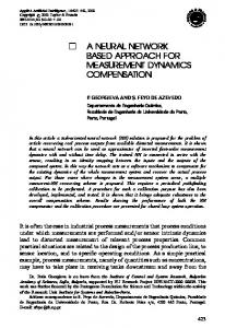
Some of these features can be observed in Fig. 1, which shows short-duration underwater signals due to a toad sh. Arti cial neural networks (ANNs) have several properties that make them promising for the automatic signal classi cation problem. They can serve as adaptive classi ers that learn through examples [5, 6]. Thus, they do not require a good apriori mathematical model for the underlying signal characteristics. This is advantageous since a comprehensive characterization of short-duration acoustic signals is not available yet. There are several neural networks that show comparable performance over a wide variety of classi cation problems, while providing a range of trade-os in training time, coding complexity and memory requirements [7, 8]. Some of these networks, including the multilayered perceptron when augmented with weight decay strategies [9], and the elliptical basis function network introduced in this paper, are quite insensitive to noise and to irrelevant inputs [10]. Moreover, a rmer theoretical understanding of the pattern recognition properties of feed-forward neural networks has emerged recently, that can relate their properties to Bayesian decision making and to information theoretic results [11, 12]. Neural networks are not \magical". They do require that the set of examples used for training should come from the same (possibly unknown) distribution as the set used for testing 1

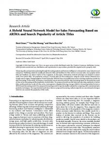
the networks, in order to provide valid generalization and good performance on classifying unknown signals [13, 14]. Also, the number of training examples should be adequate and comparable to the number of eective parameters in the neural network, for valid results [12, 15, 16]. In this context, it is noted that cross-validation techniques can partially counter the eects of small training set size [12, 17]. This paper presents the design and evaluation of a comprehensive detection and classi cation system that uses a hybrid of ANN and statistical pattern recognition techniques tailored to recognizing short-duration oceanic signals [18]. Theoretical reasoning is provided for several of the design decisions, and performance results are given for the DARPA standard data set I. Figure 2 shows the overall design of the hybrid classi er. Section 2 describes the preprocessing of the raw analog signals obtained from passive sonar and extraction of useful feature vectors from them. Our experience with alternative signal descriptors underscores the importance of selecting appropriate feature combinations in determining the classi cation quality, irrespective of the classi cation techniques used [19]. The various types of ANNs used for classi cation are described in Section 3, with particular emphasis on a novel local basis function classi er and the Pi-Sigma higher order network [20]. The DARPA standard data set I [21] is described in Section 4, and experimental results obtained by individual classi ers on this data set are presented. Section 5 introduces a high-level decision-making module which combines the evidences obtained from distinct classi ers for more accurate and robust results. Concluding remarks are given in Section 6.

2 Signal Preprocessing and Feature Extraction In order to classify events such as short-duration signals in a time series obtained from an underwater acoustic sensor, it is requisite that i) all eects that vary, but not as a result of the events of interest, be removed or accounted for to the greatest possible extent; and ii) the presence of each type of signal of interest should result in a measurable dierence in the observable features. These two requirements lead to the need for background normalization and feature extraction/selection respectively. One hallmark of our approach is that processing and classi cation is performed on all input data without the usual signal-to-noise ratio (SNR) based prescreening to select signals for classi cation.

2.1 Preprocessing The set of signal features that are extracted should be independent of the time-varying noise eld and the sensor dynamics. Since the feature vectors are typically composed of combinations of broadband and narrowband energy estimates, the signal spectrum should be whitened across the entire band. Thus, the rst step is to use an adaptive time-domain whitening lter to decorrelate the data from the long-time ambient noise, interference, and sensor characteristics, while passing short-duration signals relatively unchanged [22]. 2

After a signal is extracted and pre-whitened, there are two basic choices for representing a signal in a form suitable as inputs to a neural network classi er: (i) A signal can be represented by a single vector that encodes some features of the signal. This vector is then used as an input for a static classi er such as those described in Section 3. Previous works on sonar classi cation have most often used the normalized power spectra segmented into frequency bins (of equal or logarithmic size) to obtain the input vector. For example, input vectors based on the power spectra of passive sonar returns have been used in a multilayered perceptron network for a simple two-object problem [23], and also with a probabilistic neural network [24]. However, this simple approach is inadequate for more real-life, short-duration oceanic signals. A vector obtained from the power spectra needs to be augmented by other temporal and spectral descriptors such as signal duration, peak frequencies, bandwidths and possibly transformed AR model coecients. Another technique is to use multiscale representations such as Gabor wavelets [25] that do not require assumptions of signal stationarity. (ii) Each signal can be represented by a series of feature vectors sequenced in time [26]. Each feature vector is a descriptor of the signal observed within a particular time window. A set of overlapping time windows is used to obtain the sequence. For example, a sequence of vectors obtained by the energy in discrete frequency bins extracted through successive time windows over the input signal, can be used to form such a composite vector. Note that such representations explicitly recognize the inputs to be spatiotemporal signals, and are suited for dynamic classi ers mentioned in Section 3.1. The set of features extracted from a signal can also be regarded as a two-dimensional input for use in models such as time-delay neural networks [6].

2.2 Feature Vector Selection It was observed in our previous study [19, 21] that discriminant parameters obtained using wavelet transforms yield better performance than those using autoregressive (AR) modeling or spectral coecients. We note that both AR modeling and cepstral coecients are sensitive to the SNR of the signal, the phase, and the modeling order. Many oceanic signals are embedded in signi cant noise, mostly broadband. Phase depends on the estimated starting point of the signal, which is dicult to determine even with a good detector. Setting a high SNR threshold for lower false alarm also results in a poorer phase estimate. Finally, both broadband and narrowband signals are important, and too high an order results in noisy coecients. To extract the features, a constant-Q prototype wavelet with 24 coecients is used, in addition to signal time duration to characterize the signals in our current work. Constant-Q analysing function is broadband and of very short duration at the higher frequencies, corresponding to better SNR representation of impulsive sounds. At lower frequencies, the bandwidth is narrower and the duration longer. A good overview of wavelet transforms can be found in [27]. The particular wavelet transform used in this paper represents a signal x(t) by shifted and dilated versions of an analyzing waveform [25]: 3

Z

1 Tx(; a) = a?m=2 ?1 x(t)g( t a?m )dt

(1)

g(t) = a?m=2g( t a?m )dt

(2)

where the prototype wavelet is given by

Here a is a scaling factor, m the scaling index, and * indicates the complex conjugate. The choice of the most appropriate prototype function is still an open research issue. To date, fractional octave frequency spacing has proved quite successful. Another important classi cation parameter is the signal duration. In fact, in the DARPA Standard Data Set I, signal duration is the only discriminant between classes C and D. The duration of realistic acoustic signatures can vary over two orders of magnitude. The importance of this metric is underscored by the recent work by French researchers [28] who have used a two-stage architecture for classifying oceanic signals. The rst stage extracts the signals and sorts them into dierent categories according to signal duration. The second stage then uses a neural classi er for each category. Unfortunately, this approach is computationally expensive when there is a wide range of signal durations, and is also limited in quality of results. In the experiments reported in this paper, time duration is simply used as an added classi cation parameter. Thus the actual dimension of each feature vector is 25 (24 wavelet coecients plus time duration) when wavelet-based features are used. Irrespective of the approach taken, the use of large, possibly composite, feature vectors can become computationally expensive. If the resultant input is of high dimension, it forces us to use a network with a higher number of free or eective parameters. This leads to a classical estimation problem if the training set size is small in comparison, wherein the presence of a larger number of parameters can result in a solution that is over-determined [29]. Also, highdimensional feature vectors are more susceptible to noise. Moreover, the presence of irrelevant feature combinations can actually obscure the impact of the more discriminating inputs. An obvious solution to these problems is to reduce each feature vector to a much lower dimensional vector for actual presentation to the classi cation networks. We tried this approach by extracting the most signi cant principal components using Sanger's method [30], and also implemented a modi ed version of Kohonen's self-organizing feature maps described in [31] as an alternate technique for dimensionality reduction. Both these approaches did not fare well due to the non-stationary nature of the signal and the small size of the training set. This led us to tackle the problem with the classi cation networks themselves, by using variations of ANN classi ers that are more eective for high-dimensional inputs and more robust against noise. This issue is further discussed in Section 3.

3 Neural Network Classi ers ANN approaches to problems in the eld of pattern recognition and signal processing have led to the development of various \neural" classi ers using feed-forward networks [32, 33]. These 4

include the Multi-Layer Perceptron (MLP) as well as kernel-based classi ers such as those employing Radial Basis Functions (RBFs) [34, 35]. A second group of neural-like schemes such as Learning Vector Quantization (LVQ) have also received considerable attention [31]. These are adaptive, exemplar-based classi ers that are closer in spirit to the classical K-nearest neighbor method. The strength of both groups of classi ers lies in their applicability to problems involving arbitrary distributions. Most neural network classi ers do not require simultaneous availability of all training data and frequently yield error rates comparable to Bayesian methods without needing apriori information. Techniques such as fuzzy logic can be incorporated into a neural network classi er for applications with little training data [36]. A good review of probabilistic, hyperplane, kernel and exemplar-based classi ers that discusses the relative merit of various schemes within each category, is available in [37, 32, 33]. Comparisons between these classi ers and conventional techniques such as decision trees, K nearest neighbor, Gaussian mixtures, and CART can be found in [33, 38].

3.1 Static vs. Dynamic Approaches For all of the classi ers mentioned above, each signal needs to be represented by a single feature vector rather than as a spatiotemporal pattern that changes with time. This is why such classi ers are often referred to as \static" systems [32]. Indeed, almost all of the neural network classi ers that have been studied and used so far fall into this category. Since static classi ers are based on reduced input representations, they have an inherent drawback in that information contained in the temporal variations in the signal may not get recorded. Since many short-duration oceanic signals such as whale cries, have characteristics such as FM slides, important discriminatory evidence may be lost when each signal is represented by a single vector. This motivates the use of dynamic classi ers that base their decisions on a sequence of feature vectors corresponding to dierent, possibly overlapping, time intervals. The appropriate signal representation for such dynamic classi ers corresponds to the second choice mentioned in Section 2. A dynamic neural classi er can be implemented through recurrent networks that can store past history feedback connections among the processing cells. These networks can be used to classify waveforms of arbitrary duration using a network of xed complexity, and have been used successfully in speech recognition [6]. Dynamic recurrent networks are of three main types: (a) Partial recurrent networks using context units involve feedback to selective cells in order to record temporal sequences. Notable examples are networks that use feedback from output units to the input layer [39] or specify a context from hidden cells [40]. We observe that units with feedback connections accumulate an exponentially decaying weighted sum of current and past values to construct a static representation of a temporal input sequence. Such an architecture avoids two de ciencies found in other models of sequence recognition: rst, it reduces the diculty of temporal credit assignment by focusing the back-propagated error signal; second, it eliminates the need for a buer to hold the input sequence and/or intermediate activity levels. However, they require clocked inputs, and are susceptible to 5

spatiotemporal warping [41]. (b) Real-time recurrent backpropagation and time-dependent recurrent backpropagation [42] do not require clocked inputs, but are very sensitive to learning rates. (c) Dynamic-in-time networks that continuously update con dences of the input belonging to each class as feature vectors are presented in sequence, and makes a decision if the con dence factor exceeds a threshold for some class. We are currently investigating one such model for classifying oceanic signals. Overall, dynamic classi ers are more powerful and promising for complex temporal patterns. At present, the candidate dynamic classi ers are very susceptible to signal misalignment or registration problems and to spatiotemporal warping. They also need longer training schedules and easily exhibit divergent behavior unless the adaptation parameters are ne-tuned and the inputs have little noise components. For these reasons, we do not consider dynamic classi ers any further in this paper, while recognizing their potential.

3.2 Design Considerations and Tradeos Besides the MLP, RBF and LVQ type static classi ers mentioned above, there are several other neural-like candidates such as higher-order polynomial GMDH classi ers and functional-link networks [43, 44]. Given such a wide variety, what should be the criteria for determining the most suitable ones for classifying short-duration oceanic signals? Our experiences, corroborated by those of several other researchers (see [33] for example), show that classi cation error rates are similar across dierent classi ers when they are powerful enough to form minimum error decision regions, when they are properly tuned, and when sucient training data is available. Practical characteristics such as training time, classi cation time and memory requirements, however, can dier by orders of magnitude. Also, the classi ers dier in their robustness against noise, eects of small training sets, and in their ability to handle highdimensional inputs [10]. These factors, rather than small dierences in the best possible error rates, should form the basis of our network selection process. RBF networks are primarily aimed at multivariate function interpolation or function approximation, and have been used successfully for problems such as prediction of chaotic time series[35]. They serve as universal approximators using only a single hidden layer [45]. However, they can also be used for classi cation. For example, Niranjan and Fallside were able to achieve good results on voice and digit speech categorization by using one \centroid" for each training vector [46]. The results are robust with respect to variations in the class distributions. Thus, our rst candidate for a short-duration oceanic signal classi er is an adaptive, kernel-based network described in Section 3.3. We observe that LVQ and it variants such as LVQ2, LVQ2.1 and \conscience learning" [47] need somewhat less training time than an MLP-based classi er for comparable performance [37]. The memory requirements are similar but their performance is more sensitive to initial choice of reference vectors. Networks using RBFs, on the other hand need much shorter training times at the expense of additional memory as compared to the MLP. The localized response of hidden units in kernel-based networks such as the RBF network, as compared to 6

the global responses of MLP networks, make them suitable for detecting atypical signals or false alarms since they result in low values of network outputs. This motivates us to investigate hybrid networks that combine the best features of LVQ and RBF based classi ers so that an accurate classi er is obtained that requires less training time and is not memory intensive. A novel hybrid network that achieves these objectives is also discussed in Section 3.3, and forms our second classi er candidate. Higher-order networks based on the GMDH algorithm often require long training times as well as large amount of memory to yield comparable error rates [8]. Polynomial networks based on Volterra series expansion [48, 49] show fairly stable, single-layer learning, but the number of weights involved grows exponentially with the order of the network. We have recently proposed a higher order network called the Pi-Sigma network, that is able to maintain the capabilities of polynomial networks while greatly reducing network complexity [20, 50]. It is also able to incrementally grow till a desired level of complexity is reached. This network is the third classi er candidate, and is described brie y in Section 3.4. MLP networks that adapt weights using gradient descent of the mean squared error (MSE) in weight space, are perhaps the most commonly used neural network classi ers. These networks are capable of approximating any arbitrary bounded measurable function de ned over a compact set, given sucient number of hidden units [51]. The generalization capability of these networks can be enhanced by restricting the weight-space through adding extra terms to the cost functions or by selective pruning of weights [13, 9]. Weight pruning techniques also serve to reduce the eective number of parameters [15], making the resultant \parsimonious" feed-forward networks more tailored to noisy, high-dimensional inputs. Moreover, the rst hidden layer of an MLP can be considered as feature extractors, specially if localized connections are used. Countering the advantages of an MLP mentioned above, are the problems of high training times, and of choosing an appropriate network size. As noted by Makhoul [12], \the sigmoid, because of its sharp transition ... focuses attention during training on data samples that are confusable. Basically, it helps specify the boundary between the samples within and outside the class. Thus, in general, much of the training data does not participate in determining the network parameter values." We note that this drawback is even more severe when the number of training samples is limited. For all these reasons, the MLP is not considered further in this paper, and instead the reader is referred to [52] for our results on using an MLP with optimal brain damage [9] for classifying underwater signals from biologic sources.

3.3 Ecient Adaptive Kernel Classi ers We rst summarize the LVQ and RBF procedures and then introduce two hybrid networks that attempt to incorporate the best of both LVQ and RBF techniques. LVQ is an adaptive version of the classical Vector Quantization algorithm whose aim is to represent a set of input vectors by a smaller set of codebook vectors or reference vectors (RVs) so as to minimize an error functional. Typically, the algorithm consists of the following 7

steps: The RVs are initialized by a random selection or from K-means clustering on the training set. These vectors are now adjusted iteratively by moving them closer to or further away from training inputs depending on whether the closest RV is of the same class as the input vector or not. Unknown inputs are assigned the class of the nearest RV, with the Euclidean norm being the most common measure of distance. Let the nth training pattern vector x(n) belong to class Cr , and mc(n), the reference vector closest to x(n), belong to class Cs. At the presentation of the nth input, the RVs are adapted as follows.

mc(n + 1) = mc(n) + (n)[x(n) ? mc(n)] if Cr = Cs mc(n + 1) = mc(n) ? (n)[x(n) ? mc(n)] if Cr 6= Cs mi(n + 1) = mi(n) for all other RVs

(3)

where (n) is a learning factor that decreases monotonically with time. Details of LVQ-type learning procedures can be found in [47, 31, 53]. RBF networks are a class of single hidden-layer feedforward networks in which radially symmetric basis functions are used as the activation functions for the hidden layer units. A generic RBF network is shown in Fig. 3. Let xp = (xp1; xp2; : : :; xpN )T denote the pth Ndimensional input. When this input is presented to the RBF network, the output of the j th hidden node, Rj (xp), and that of the ith output node, fi(xp), are given by :

X w R (x ); ij j p

(4)

Rj (xp) = R( kxp ? xjk );

(5)

fi(xp) =

j

j

where R(
) is a radially symmetric function such as a Gaussian. In the above, xj is the location of the j th centroid, where each centroid is a kernel/hidden node, j is a scalar denoting the \width" of its receptive eld and, wij is the weight connecting the j th kernel/hidden node to the ith output node. For Gaussian RBFs, the width j is the standard deviation, so that we have kxp ?xj k ?  Rj (xp) = e : 2

1 2

2

Hybrid Kernel Classi ers: Both LVQ and RBF involve construction of a representative set of the training data - the centroids or hidden units of RBF and the reference vectors of LVQ - which determine the nal decision. Previously, the centroids in an RBF network were determined using heuristics such as performing k-means clustering on the input set, and widths were held xed during training. Alternatively, we can vary both the centroid locations and associated widths of the receptive elds by performing gradient descent on the mean square error of the output. This leads to the Adaptive Kernel Classi er (AKC). P Ep, where Adaptive Kernel Classi er: Consider a quadratic error function, E = p Ep = 21 Pi(tpi ? fi(xp))2. Here tpi is the ith component of the target function for input xp, and fi(xp) is the corresponding network output as de ned in Eq. 4. The mean square error is 8

the expected value of Ep over all patterns. Let
wij ;
xjk and
j represent the change in weight wij , location of kth component of the j th centroid, and the width, j of this centroid respectively, at each learning step. The update rules for these network parameters are obtained using gradient descent on Ep, and are given by:
wij = 1(tpi ? fi(xp))Rj (xp);

X


xjk = 2Rj (xp) (xpk ?2 xjk ) ( (tpi ? fi (xp))wij ); j

i

X


j = 3Rj (xp) kxp ?3xjk ( (tpi ? fi(xp))wij ): 2

j

i

(6) (7) (8)

These equations constitute the learning scheme for the Adaptive Kernel Classi er. A similar scheme, called the Gaussian Potential Function Network (GPFN), which involves segmentation of the input domain into several potential elds in form of Gaussians, was proposed by Lee and Kil [54]. The Gaussian potential functions of this scheme need not be radially symmetric functions. Instead, the sizes of these potential elds are determined by a correlation matrix. The network parameters are computed by gradient descent as in the case of AKC. We studied a network of nonradial basis functions with a dierent smoothing factor in each dimension. Thus, Eq. 4 is used with

Rj (xp) = e

? 21 k (xpk?2xjk ) jk

2

;

(9)

and, in general, jk 6= jl. For this case update rules (7) and (8) become,

X


xjk = 2Rj (xp) (xpk?2 xjk ) ( (tpi ? fi(xp))wij ) jk

i

X


jk = 3Rj (xp) (xpk ?3 xjk ) ( (tpi ? fi(xp))wij ): 2

jk

i

(10) (11)

Classi cation experiments show that these Elliptical Basis Function Networks require considerably shorter training times compared to the AKC and typically require a fewer number of kernel nodes. To further speedup network training, we suggest replacement of the parameter  with a new parameter  by making the substitution  = 1=. This eliminates all division operations involved in training and testing, which are known to be computationally expensive. How should the widths, jk s be initialized? For RBF, the initial positions of the centroids are typically obtained by k-means clustering, and the width j for the j th centroid is of the same order as the distance between this unit and the nearest centroid, xj . This suggests the initialization

jk (init) =   kxj ? xj k; 8j; k: 9

However, since the spread of data is is general dierent in dierent dimensions, an initialization given by: jk (init) = n1=2  kxjk ? xjkk; 8j; k: seems more appropriate, where  = O(1) determines selectivity, and n1=2 is a normalization term for n-dimensional inputs so that the average variance is j2, as before. More general schemes like the regularization networks have been studied by Poggio et al. [55]. Though more complex decision regions can be shaped out of potential elds that are not radially symmetric, receptive elds of radial functions can achieve universal approximation even if each kernel node has the same smoothing factor,  [56]. The principal advantage of the AKC is that it is able to perform the same level of approximation as RBF using fewer hidden units. However, training time is increased since centroids and center widths are also adapted using the generalized delta rule, which is a slower procedure. Rapid Kernel Classi er: Hybrid schemes which combine unsupervised and supervised learning in a single network have been proposed in [57], [5]. For instance, the hierarchical feature map classi er of Huang and Lippmann [5] consists of a feature map stage followed by a stage of adaptive weights. The central idea behind these approaches is to have a layer that is trained in an unsupervised way followed by a layer that will be trained using the delta rule. Since backpropagation of error through multiple layers is avoided these hybrid networks yield remarkable speedups in computation. Such methods are particularly useful when there are a large number of training samples. It must be noted that these hybrid schemes are not optimized in the manner of backpropagation since the rst stage parameters are not optimized with respect to the output performance. A question that immediately arises is: how does the location of centroids obtained by hybrid training compare with that obtained by strict gradient descent? Keeping in view the similarities in form between the equations describing update of centroids by the delta rule and the LVQ algorithm, one can replace the former equation with the latter in the AKC training scheme. This results in the Rapid Kernel Classi er (RKC) shown in Fig. 4, which requires shorter training times with little change in performance as compared to the Adaptive Kernel Classi er. In the hybrid procedures mentioned above various layers of the network are trained sequentially. The rst stage parameters are rst trained in an unsupervised way and are held xed during the second stage training. On the contrary, in the RKC scheme we let the LVQ algorithm run in parallel with the training of the second layer. We note that a variant, RKCEB, can also be studied in which elliptical basis functions are used. Interestingly, in all our experiments so far with RKC, the mean square error decreases monotonically as in the case when all the parameters are adapted by backpropagation. This indicates that adjusting the centroids using LVQ might amount to performing gradient descent on the \centroid-location space". While proving this seems dicult, we have been able to obtain preliminary results indicating such a connection [58]. The distinguishing features of the various localized networks introduced in this section are summarized below: 10

Type

Adaptation of Network Parameters Centroid Weights Widths RBF K-means/ xed Delta rule Fixed; isotropic AKC Delta rule Delta rule Delta rule; isotropic EBF Delta rule Delta rule Delta rule; anisotropic RKC LVQ Delta rule Delta rule; isotropic RKCEB LVQ Delta rule Delta rule; anisotropic

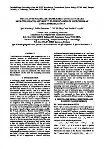
3.4 Higher-Order Pi-Sigma Networks The recently introduced Pi-Sigma networks (PSNs) [20, 50] are higher-order network whose name stems from the fact that these networks use products of sums of input components instead of sums of products as in \sigma-pi" units, to obtain the outputs. The primary motivation for these networks is to develop a systematic method for maintaining the fast learning property and powerful mapping capability of single layer higher-order networks while avoiding the combinatorial increase in the number of weights and processing units required. Figure 5 shows a Pi-sigma Network (PSN) with a single output. This network is a fully connected two-layered feedforward network. However, the summing layer is not \hidden" as in the case of the multilayered perceptron (MLP), since weights from this layer to the outputs are xed at 1. This property drastically reduces training time. Let x = (1; x1; : : :; xN )T be an N + 1-dimensional augmented input column vector where xk denotes the k-th component of x. The inputs are weighted by K weight vectors wj = (w0j ; w1j ; : : : ; wNj )T ; j = 1; 2;


; K and summed by a layer of K linear \summing" units, where K is the desired order of the network. The output of the j -th summing unit, hj , is given by:

hj = The output y is given by:

N X wkj xk + w0j ; j = 1; 2; : : : ; K:

k=1

YK

y = f ( hj ); j =1

(12) (13)

where f (
) is a suitable nonlinear activation function, and is chosen as the sigmoid function: f (x) = 1 +1e?x ; (14) for our purposes. In Eqs. 12,13, wkj is an adjustable weight from input xk to j -th summing unit and w0j is the threshold of the j -th summing unit. The weights can take arbitrary real values. If a speci c input, say, xp is considered, then the (hj )'s, y, and net are superscripted by p. The network shown in Figure 5 is called a K -th order PSN since K summing units are incorporated. The total number of adjustable weight connections for a K -th order PSN 11

with N dimensional inputs is (N + 1)
K . If multiple outputs are required, an independent summingPlayer is needed for each output. Thus, for an M -dimensional output vector y, a total of Mi=1(N + 1)
Ki adjustable weight connections are needed, where Ki is the number of summing units for the i-th output. This allows us great exibility since all outputs do not have to retain the same complexity. Note that using product units in the output layer indirectly incorporates the capabilities of higher-order networks with a smaller number of weights and processing units. This also enables the network to be regular and incrementally expandable, since the order can be increased by one by adding another summing unit and associated weights, but without disturbing any connection established previously. An asynchronous adaptation rule is used in which only those weights corresponding to the lth summing, randomly chosen for each input, is updated per input sample. Such a rule leads to more stable learning than updating all weights at each step. Gradient descent on the estimated MSE leads to the following update rule: Y
wl = 
(tp ? yp)
(yp)0
( hpj)
xp; (15) j 6=l

where (yp)0 is the rst derivative of sigmoidal function (
), xp is the (augmented) p-th input pattern and  is the learning rate. PSNs have been successfully applied to several problems involving function approximation or pattern classi cation. A second or third order network is usually sucient for obtaining a reasonably good decision surface in very short time. Another advantage is that more dicult signals can use a network with more summing units, without disturbing the smoother lower-order generalization for simpler signal classes. The behavior of PSNs is well characterized mathematically, and bounds on the learning rate,  for convergence, can be found in [50].

3.5 Statistical Classi ers Besides the neural network classi ers, we also considered several traditional classi ers based on the theory of statistical pattern recognition [59, 60]. The rst is the K-Nearest Neighbor (KNN) classi er which is a kernel-based technique. The KNN assigns to an unclassi ed data sample the identity of the majority of the nearest (in a Euclidean sense) K preclassi ed samples from the training data. While the error rate is typically greater than the Bayes optimal risk, the KNN error is bounded by twice the Bayes optimal risk. Since our number of training samples per class ranged from 5 to 9, K = 3 was chosen. Note that since every training sample has to be considered in the labeling process, the memory and computational requirements increase linearly with the training data size. Also, this technique cannot dierentiate among simultaneously occurring signals since it does not decompose an input vector. The second classi er considered is the generalized Fisher Linear Discriminant, often referred to as the Linear Classi er (LC). The LC uses the lumped covariance matrix, R, and the individual class dependent means, Mj to compute V (j; X ) = (X ? Mj )T R?1 (X ? Mj ) (16) 12

for each class, and declares the membership of input X to be same as that j for which the value of V (j; X ) is the least. For the short duration signals in the DARPA Standard Data Set I, singularities in R were found. These were handled using Singular Value Decomposition techniques to perform the matrix inversion and a step-wise regression to determine good features. Although the LC is easy to use, it is cumbersome to update, and degrades rapidly as the Bayes optimal decision boundaries become highly non-linear. The performance of the LC is given in [21], and is not repeated here because it is inferior to all the other techniques considered. Similarly, the results of using a quadratic classi er are omitted since they were much more computationally intensive without showing a signi cant improvement in classi cation accuracy as compared to the LC.

4 Performance Evaluation 4.1 Data Description and Representation The various classi ers described in the previous section have been evaluated for their ability to classify short duration acoustic signals extracted from DARPA Standard Data Set I [18]. This data set consists of digital time records of a training and a test set of 6 signal types propagated over short oceanic data paths with variable source and background noise levels. For the results reported in this paper, only those portions of the records that contain signals are used. As shown in Table 1, the 6 signal classes are denoted by the letters A through F with durations from a few msec to 8 seconds, and bandwidths from less than 1 Hz to several kHz. The signal to noise ratios of the records vary over 24 dB. There were 42 training samples. Of the test data, 179 samples were similar enough to the training data to constitute a good test set for classi cation comparisons. An additional 19 test samples were added selectively to observe, without retraining, the robustness of the techniques to extraneous deterministic signals. These 19 additional records had duration and frequency characteristics that deviated signi cantly from the training data, and are thus identi ed by primed labels in Table 1. Overall, the data set included several signal characteristics that are representative of realistic oceanic signals, including (i) Simultaneously occurring signals (some type F signals, several type B signals). (ii) Sequentially occurring signals requiring event association. (iii) Signals similar to type C or type A but with some important feature missing. (iv) Signi cant signal variations due to the source or propagation path; possibly low SNR.

13

Table I. DESCRIPTION OF DARPA STANDARD DATA SET I Signal Classes Number of Samples Class Description Training Test 179 Additional 19 Deviant Test Signals A Broadband, 15 msec pulse 7 53 8 (A0) B Two 4 msec pulses, 27 msec separation 7 54 6 (B 0 ) C 3 kHz tonal, 10 msec duration 8 31 1 (C 0) D 3 kHz tonal, 100 msec duration 9 14 0 (D0 ) E 150 Hz tonal, 1 sec duration 6 19 4 (E 0) F 250 Hz tonal, 8 sec duration 5 8 0 (F 0 ) TOTALS 42 179 19 From the size of the training set, it is apparent that the training data is small compared to the number of free parameters for all of the neural networks considered, with the problem being most severe for the basis function networks and least for the Pi-Sigma network. This sparse data problem is dealt with by using cross-validation, wherein part of the training data is also used to test the network at every training cycle, and training is stopped when the performance reaches a peak and begins to fall. In this way, the network is encouraged not to memorize the training data, and can do better generalization when faced with unknown data.

4.2 Performance of Individual Classi ers The adaptive and rapid kernel classi ers were compared with the LVQ2 and RBF, as well as the K-Nearest Neighbor (KNN) classi er and the Pi-Sigma higher order network [20] in terms of classi cation accuracy, training and test times, and memory requirements. The LVQ2 and the two hybrid algorithms used 5 reference vectors for each class, while the RBF used a total of 15 centroids. For the KNN, K = 3 was chosen, and the number of training samples ranged between 5 and 9 per class for a total of 42 samples. The Pi-Sigma network used 3 hidden units, and was trained using all 42 samples. The number of iterations, determined by a cut-o in dierential MSE of 0.001 was 35, 104 and 816 for the RKC, AKC and Pi-Sigma networks respectively. The classi cation results for the six dierent techniques, examined only for the signal epochs, are displayed in Figure 6 using confusion matrices. For each technique, the correct class is given by the horizontal row label and the misclassi cation (or confused) class assigned is given by the vertical column label. The numerical entries give the number of misclassi cations. Such a display format exposes which signals cause the greatest problems for a given technique. The upper half of the matrix shows the results for the 179 test signals, while the lower half, identi ed by the primed labels A0 through E 0, display results for the 19 deviant test signals. We note that the AKC is able to classify all regular test signals correctly (100%) while the 3-NN gave the poorest results (7 misclassi cations or 96.1% accuracy). For the deviant signals, all six techniques could label only 4 to 6 (21.1% 31.6%) in agreement with the provided ground truth. The dramatic contrast in performance for the additional 19 test signals indicates that the classi ers were sharply tuned to the deterministic- like signals of the training set and not amenable to grossly deviant signals. This conclusion is further reinforced by interpreting the network outputs, as elaborated below. Besides classi cation accuracy, memory requirements, training and testing times are also of concern, particularly for real-time implementations. The AKC took the longest training time, while

14

the RKC was quicker than LVQ but provided superior results. While determining the class of a test signal, the Pi-Sigma and RBF networks are about twice as fast than the other networks which exhibit comparable speeds. More accurate timing estimates could be obtained through a careful separation of CPU and input/output times.

5 Evidence Integration and Decision Making We observe that the DARPA Standard Data Set I is a simpli ed characterization of real-life, shortduration oceanic signals, whose detection and classi cation is a much more dicult problem. Since dierent classi cation techniques have dierent inductive biases, a single method cannot give the best results for all signal types. Rather, more accurate and robust classi cation can obtained by combining the outputs (evidences) of multiple classi ers based on neural network and/or statistical pattern recognition techniques. With this motivation, we present two such techniques for evidence combination in this section. It has been recently shown that training multilayer feedforward networks by minimizing the expected mean square error (MSE) at the outputs and using a 0/1 teaching function yields network outputs that approximate posterior class probabilities [61, 62, 63]. In particular, the MSE is shown to be equivalent to

MSE = K1 +

XZ

x

c

Dc (x)(P (c=x) ? fc(x))2dx

(17)

where K1 and Dc (x) depend on the class distributions only, fc (x) is the output of the node representing class c given an input x, P (c=x) denotes the posterior probability, and the summation is over all classes. Thus, minimizing the (expected) MSE corresponds to a weighted least squares t of the network outputs to the posterior probabilities. This result gives a sound mathematical basis for the interpretation of the network outputs, and for using an integrator to combine the outputs from multiple classi ers to yield a more accurate classi cation. For very low values of MSE, fc (x) approximates P (c=x) according to Eq. 17. Let fc;i(x) be the output of the node that denotes membership in class c in the ith neural classi er. We expect that, for all i, x :

Xf c

c;i = 1:

(18)

Similarly, if the posteriori estimate is very good, one would expect for all c; i: N 1X N fc;i (xj ) = P (c); j =1

(19)

where j indexes the N training data samples, and P(c) is obtained by counting the frequency of class c in the training data. Indeed, both Eq. 18 and Eq. 19 are observed to be quite accurate for almost all of the 179 test signals for both RKC and AKC, as well as for the Pi-Sigma network. For 16 of the 19 deviant signals, the summation of Eq. 18 is less than 0.5, strongly indicating that these signals do not resemble any signal in the training set.

15

Based on the interpretation of the outputs as aposterior class probabilities, two methods for evidence combination were proposed and used [52]: 1. Entropy-Based Integrator. In this method, a weighted average of the outputs of n dierent classi ers is rst performed, with a larger entropy resulting in a smaller weight. The integrator then selects the class corresponding to the maximum value, providing this value is above a threshold. Otherwise, the input is considered as a false alarm, since there is no strong evidence that it belongs to any of the n classes. 0 = yc;i = P yc;i . First, for every classi er, the entropy is calculated using normalized outputs yc;i c The weight given to each classi er (normalized) output diers from sample to sample according to the (approximated) entropy at the output of that classi er, as follows:

H (c) = n1

Xn P yc;i ? c y0 ln y0 c;i

i=1

c;i

;

assigned class label = c : max H (c): (20) In this way, the outputs of a classi er with several similar values get a lower weighting as opposed to classi ers which strongly hypothesize a particular class membership. Our initial experiment in combining the results of the RKC and the Pi-Sigma network yielded 100% accuracy among the 179 test signals and 8/19 (42%) agreement with the ground truth provided for the deviant signals. More signi cantly, the values of max fH(c)g obtained for this set are signi cantly lower, thus indicating that this metric can be used to detect false alarms and unknown signals. 2. Heuristic Combination of Con dence Factors. This approach is inspired by techniques for parallel combination of rules in expert systems. Certainty factors were introduced in the MYCIN expert system for reasoning in expert systems under uncertainty, and re ect the con dence in a given rule [64]. The original method of rule combination in MYCIN was later expressed in a more probabilistic framework by Heckerman [65], and serves as the basis for the method proposed below: First, the outputs, which are in the range [0,1], are mapped into certainty or con dence factors (CFs) in the range [-1,1] using a log transformation. Then, a MYCIN-type rule is used to combine the CFs for each class. The advantage of this combination rule is that it makes the result invariant to the sequence in which the dierent network outputs are combined. The individual CFs are rst obtained using: CFc;i = logn((n ? 1=n)yc;i + 1=n); (21) where subscript i denotes the classi er as before. For each class c, all positive CFs and all negative CFs are combined separately. The resultant positive and negative CFs are combined in the nal step, to obtain a combined con dence CFc , for each class c. The classi cation decision is: assigned class label = c : max CFc : The equations used for combining the CFs are similar but not identical to those used in the original MYCIN [64]. For a given class, c, let the individual con dences obtained from two classi ers be a and b respectively. Then the con dence Cc (a; b) obtained on combining these two values, is given by: CFc(a; b) = 1 ? (1 ? a)(1 ? b) if a > 0 and b > 0; (22) = ?CFc (?a; ?b) if a < 0 and b < 0; = a + b; otherwise:

16

An experiment in combining the results of the RKC and the Pi-Sigma network using con dence factors also yielded 100% accuracy among the 179 test signals and 9/19 (47%) agreement with the ground truth provided for the deviant signals. Again, the values of max CFc were much lower for the deviant signals, yielding another metric for detecting false alarms and unknown signals. Indeed, by varying the threshold for the minimum acceptable value for max H (c) or max CFc , one can obtain a range of classi cation accuracy versus false alarm rates, and be able to choose a suitable trade-o point.

6 Concluding Remarks Hybridization of algorithms is emerging as an important approach to solving problems. Each algorithm is a realization of one approach to a solution, and often a synergistic approach to the problem yields a better solution than making further improvements on a single approach. In fact, increasing the sophistication of a particular technique may not take us very far, as is witnessed by the history of LVQ. Rather, for dicult real-world problems like detection and classi cation of oceanic signals, it is crucial to have good preprocessing and feature selection techniques combined with ecient neural network classi ers and robust methods for integrated decision-making. Good performance is required at every stage, and cooperation is also desirable between stages. In our classi er, these principles are exempli ed by the coupling of the selection of feature vectors with the choice of neural classi ers, and by the use of evidence combination techniques in a situation when the capabilities of a single classi er are fundamentally limited. Acknowledgements: This research was supported by contract N0001489-C-0298 with Dr. Thomas McKenna (ONR) and Dr. Barbara Yoon (DARPA) as Government cognizants. We also thank James Whiteley and Russell Still at Tracor Applied Sciences, Inc., and the University of Texas team of J.K. Aggarwal, Srinivasa Chakravarthy, Chen Chau Chu, Ed Powers, Irwin Sandberg and Yoan Shin for contributions at various stages of the project.

References [1] L. Deuser and D. Middleton. On the classi cation of underwater acoustic signals: An environmentally adaptive approach. The Acoustic Society of America, 65:438{443, 1979. [2] C.H. Chen. Automatic recognition of underwater transient signals-a review. In Proc. ICASSP, pages 1270{1272, 1985. [3] Special Issue. Underwater acoustic signal processing. IEEE Jl. on Ocean Engineering, pages 2{278, January 1987. [4] R.J. Urick. Principles of Underwater Sound. McGraw-Hill(2nd Ed.), 1975. [5] W.Y. Huang and R.P. Lippmann. Neural network and traditional classi ers. Neural Information Processing Systems, pages 387{396, 1987. [6] R. P. Lippmann. Review of neural networks for speech recognition. Neural Computation, 1(1):1{ 38, 1989.

17

[7] J. Ghosh and K. Hwang. Mapping neural networks onto message-passing multicomputers. J. of Parallel and Distributed Computing, 6:291{330, April, 1989. [8] K. Ng and R.P. Lippmann. Practical characteristics of neural network and conventional pattern classi ers. In Advances in Neural Information Processing Systems -3, pages 970{976, 1991. [9] Yann Le Cun, J.S. Denker, and S. A. Solla. Optimal brain damage. In Advances in Neural Information Processing Systems -2, pages 598{605, 1990. [10] S. Beck and J. Ghosh. Noise sensitivity of static neural classi ers. In SPIE Conf. on Applications of Arti cial Neural Networks SPIE Proc. Vol. 1709, Orlando, Fl., April 1992. [11] D. Lowe and A. R. Webb. Optimized feature extraction and the bayes decision in feed-forward classi er networks. IEEE Trans. PAMI, 13:355{364, April 1991. [12] J. Makhoul. Pattern recognition properties of neural networks. In Proc. 1st IEEE Workshop on Neural Networks for Signal Processing, pages 173{187, Sept 1991. [13] J. Denker et al. Large automatic learning, rule extraction and generalization. Complex Systems, 1:877{922, 1987. [14] E. Levin, N. Tishby, and S. A. Solla. A statistical approach to learning and generalization in layered neural networks. Proc. IEEE, 78(10):1568{74, Oct 1990. [15] J.E. Moody. Note on generalization, regularization and architecture selection in nonlinear learning systems. In IEEE Workshop on Neural Networks for Signal Processing, pages 1{10, 1991. [16] P.J. Werbos. Links between arti cial neural networks and statistical pattern recognition. In I.K. Sethi and A. Jain, editors, Arti cial Neural Networks and Statistical Pattern Recognition, pages 11{32. Elsevier Science, Amsterdam, 1991. [17] S. Raudys and A.K. Jain. Small sample size problems in designing arti cial neural networks. In I.K. Sethi and A. Jain, editors, Arti cial Neural Networks and Statistical Pattern Recognition, pages 33{50. Elsevier Science, Amsterdam, 1991. [18] J. Ghosh et al. Adaptive kernel classi ers for short-duration oceanic signals. In IEEE Conf. on Neural Networks for Ocean Engineering, pages 41{48, August 1991. [19] J. Ghosh, L. Deuser, and S. Beck. Impact of feature vector selection on static classi cation of acoustic transient signals. In Government Neural Network Applications Workshop, Aug 1990. [20] Y. Shin and J. Ghosh. The pi-sigma network: An ecient higher-order network for pattern classi cation and function approximation. In Proceedings of the International Joint Conference on Neural Networks, Seattle, pages I:13{18, Seattle, WA, July 1991. [21] S. Beck, L. Deuser, R. Still, and J. Whiteley. A hybrid neural network classi er of short duration acoustic signals. In Proc. IJCNN, pages I:119{124, July 1991. [22] B. Widrow and S.D. Stearns. Adaptive Signal Processing. Prentice-Hall, Englewood Clis, N.J., 1985. [23] R. P. Gorman and T. J. Sejnowski. Analysis of hidden units in a layered network trained to classify sonar targets. Neural Networks, 1:75{89, 1988.

18

[24] J. Specht. Probabilistic neural networks. Neural Networks, 3:45{74, 1990. [25] J.M. Combes, A. Grossman, and Ph. Tchamitchian (Eds.). Wavelets: Time-Frequency Methods and Phase Space. Springer-Verlag, 1989. [26] Y.H. Pao, T.L. Hemminger, D.J. Adams, and S. Clary. An episodal neural-net computing approach to the detection and interpretation of underwater acoustic transients. In Conf. on Neural Networks for Ocean Engineering, pages 21{28, 1991. [27] O. Rioul and M. Vetterli. Wavelets and signal processing. IEEE Signal Processing Magazine, pages 14{38, October 1991. [28] T. Lefebvre, J.M. Nicolas, and P. Degoul. Numerical to symbolical conversion for acoustic signal classi cation using a two-stage neural architecture. In Proc. Int. Neural Network Conf., Paris, pages 119{122, June 1990. [29] S. Geman, E. Bienenstock, and R. Doursat. Neural networks and the bias/variance dilemma. Neural Computation, 4(1):1{58, 1992. [30] T. D. Sanger. Optimal unsupervised learning in a single-layer linear feedforward neural network. Neural Networks, 2:459{474, 1989. [31] T. Kohonen. Self-Organization and Associative Memory. Springer-Verlag, Berlin, 3rd Ed. 1989. [32] R. P. Lippmann. Pattern classi cation using neural networks. IEEE Communications Magazine, pages 47{64, Nov 1989. [33] R. P. Lippmann. A critical overview of neural network pattern classi ers. In IEEE Workshop on Neural Networks for Signal Processing, 1991. [34] D.S. Broomhead and D. Lowe. Multivariable functional interpolation and adaptive networks. Complex Systems, 2:321{355, 1988. [35] J. Moody and C. J. Darken. Fast learning in networks of locally-tuned processing units. Neural Computation, 1(2):281{294, 1989. [36] P.K. Simpson. Fuzzy min-max classi cation with neural networks. In IEEE Conf. on Neural Networks for Ocean Engineering, pages 291{300, August 1991. [37] T. Kohonen, G. Barna, and R. Chrisley. Statistical pattern recognition with neural networks: Benchmarking studies. In IEEE Annual Int'l. Conf. on Neural Networks, July 1988. [38] S. M. Weiss and C.A. Kulikowski. Computer Systems That Learn. Morgan Kaufmann, 1991. [39] M.I. Jordan. Serial order: A parallel, distributed processing approach. In J.L. Elman and D.E. Rumelhart, editors, Advances in Connectionist Theory: Speech. Lawrence Erlbaum, Hillsdale, 1989. [40] J.L. Elman. Finding structure in time. Cognitive Science, 14:179{211, 1990. [41] R. Hecht-Nielsen. Neurocomputing. Addison Wesley, 1990. [42] M. Sato. A real time learning algorithm for recurrent analog neural networks. Biological Cybernetics, 62:237{241, 1990.

19

[43] A. G. Ivakhnenko. Polynomial theory of complex systems. IEEE Transactions on Systems, Man, and Cybernetics, 1(4):364{378, October 1971. [44] Y.-H. Pao. Adaptive Pattern Recognition and Neural Networks. Addison-Wesley, 1989. [45] J. Kowalski, E. Hartman, and J. Keeler. Layered neural networks with gaussian hidden units as universal approximators. Neural Computation, 2:210{215, 1990. [46] M. Niranjan and F. Fallside. Neural networks and radial basis functons in classifying static speech patterns. Tech. Rep. CUED/FINFENG/TR22, Cambridge University Engg. Dept., 1988. [47] D. deSieno. Adding conscience to competitive learning. In IEEE Annual Int'l. Conf. on Neural Networks, pages 1117{1124, 1988. [48] C. L. Giles and T. Maxwell. Learning, invariance, and generalization in a high-order neural network. Applied Optics, 26(23):4972{4978, 1987. [49] M. R. Lynch and P. J. Rayner. The properties and implementation of the non-linear vector space connectionist model. In Proc. First IEE International Conference on Arti cial Neural Networks, pages 184{190, October 1989. [50] J. Ghosh and Y. Shin. Ecient higher-order networks for function approximation and classi cation. International Journal of Neural Systems, 3(4):323{350, 1992. [51] K. Hornik, M. Stinchcombe, and H. White. Multilayer feedforward networks are universal approximators. Neural Networks, 2:359{366, 1989. [52] J. Ghosh, S. Beck, and C.C. Chu. Evidence combination techniques for robust classi cation of short-duration oceanic signals. In SPIE Conf. on Adaptive and Learning Systems, SPIE Proc. Vol. 1706, pages 266{76, Orlando, Fl., April 1992. [53] S. Geva and J. Sitte. Adaptive nearest neighbor classi cation. IEEE Transactions on Neural Networks, 2(2):318{322, 1991. [54] Sukhan Lee and Rhee M. Kil. Multilayer feedforward potential function network. In Proceedings of the Second International Conference on Neural Networks, pages 161{171, 1988. [55] T. Poggio and F. Girosi. Networks for approximation and learning. Proc. IEEE, 78(9):1481{97, Sept 1990. [56] J. Park and I.W. Sandberg. Universal approximation using radial basis function networks. Neural Computation, 3(2):246{257, Summer 1991. [57] R. Hecht-Nielsen. Counterpropagation networks. Applied Optics, 26:4979{4984, 1987. [58] S. Chakravarthy, J. Ghosh, L. Deuser, and S. Beck. Ecient training procedures for adaptive kernel classi ers. In Neural Networks for Signal Processing, pages 21{29. IEEE Press, 1991. [59] R. O. Duda and P. E. Hart. Pattern Classi cation and Scene Analysis. Wiley, New York, 1973. [60] K. Fukunaga. Introduction to Statistical Pattern Recognition. (2nd Ed.), Academic Press, 1990. [61] M.D. Richard and R.P. Lippmann. Neural network classi ers estimate bayesian a posteriori probabilities. Neural Computation, 3(4):461{483, 1991.

20

[62] H. Gish. A probablistic approach to the understanding and training of neural network classi ers. In Proc. Int'l Conf. on ASSP, Albuquerque,NM, pages 1361{1364, April 1990. [63] P.A. Shoemaker, M.J. Carlin, R.L. Shimabukuro, and C.E. Priebe. Least squares learning and approximation of posterior probabilities on classi cation problems by neural network models. In Proc. 2nd Workshop on Neural Networks, WNN-AIND91,Auburn, pages 187{196, February 1991. [64] E.H. Shortclie and B.G. Buchanan. A model of inexact reasoning in medicine. Mathematical Biosciences, 23:351{379, 1975. [65] D. Heckerman. Probabilistic interpretation for MYCIN's uncertainty factors. In L.N Kanal and J.F. Lemmer, editors, Uncertainty in Arti cial Intelligence, pages 167{196. North-Holland, 1986.

21

Figure 1: Underwater acoustic signals due to a toad sh, displayed as time waveforms (above) and as a time-frequency spectrogram (below). The occurrence of a shorter duration signal (at around t = 1.3 sec) after the rst signal of longer duration and lower frequency band, is characteristic of toad shes. The association of these two events, together with some other signal features, enables one to distinguish toad shes from other marine biological sources.

22

Figure 2: Overall design of the signal detection and classi cation system.

23

Figure 3: A radial basis function (RBF) network.

Figure 4: A rapid kernel classi er (RKC).

24

Figure 5: A pi-sigma network with one output.

25

Figure 6: Confusion matrices showing classi cation error results for (clockwise from top left) (a) 3-Nearest Neighbor, (b) RBF, (c) LVQ2, (d) Pi-Sigma Network, (e) Rapid Kernel Classi er, and (f) Adaptive Kernel Classi er. The primed class labels shown at the bottom half of each display denote additional errors due to deviant signals.

26