hybrid wavelet artificial neural network model for ... - Semantic Scholar

VOL. 7, NO. 8, AUGUST 2012

ISSN 1819-6608

ARPN Journal of Engineering and Applied Sciences ©2006-2012 Asian Research Publishing Network (ARPN). All rights reserved.

www.arpnjournals.com

HYBRID WAVELET ARTIFICIAL NEURAL NETWORK MODEL FOR MUNICIPAL WATER DEMAND FORECASTING 1

Jowhar R. Mohammed1 and Hekmat M. Ibrahim2 Water Resources Engineering, Faculty of Engineering and Applied Science, University of Dohuk, Dohuk, Iraq 2 Dams and Water Resources Engineering, Faculty of Engineering, University of Sulaimani, Iraq E-Mail: [email protected]

ABSTRACT In this research, a hybrid model has been developed for municipal water demand forecasting based on the wavelet and artificial neural network methods. The developed model combines the discrete wavelet transforms (DWT) with multilayer perceptron neural network (MLP) called Wavelet-ANN. In order to assess the credibility of developed model results, the model was run over the available data which include the time series of daily and monthly municipal water consumption for fourteen years (1/1/1992 - 31/12/2004) of Tampa city, USA. In the developed model, the Daubechies wavelet function with different orders and levels of resolution were used in the decomposing process of time series. The approximation and each detail of the decomposed water consumption time series were modeled using the MLP neural network. It is quite clear from the results obtained from both daily and monthly forecasting models for municipal water consumption time series considered in this research that the hybrid Wavelet-ANN approach provides accurate daily and monthly forecasts as measured using a validation period of 5, 10 and 15 for daily data and 24 months for monthly data, recording MAPE values (≤ 1.029%) and R2 values (≥ 0.967). Keywords: water demand, forecasting, wavelets.

INTRODUCTION The scarcity of water is considered the most challenging problem that is facing the countries in the world. The long term forecasting of municipal water demand in such countries is a critical and essential factor for water supply planning, which includes the determining of type, size, location and timing of the required improvements and developments of the water supply systems. On the other hand, short term forecasting of municipal water demand is required for water utilities to proactively optimize pumping and treatment operations to minimize energy, water supply and treatment costs while maintaining a reliable and high quality product for their customers. There are considerable amounts of published material dealing with water demand forecasting, all of which cannot be reviewed here. However, some principal contributions of historical interest will be cited. In the last few decades there has been a growing scientific interest in the development and use of water consumption forecasting models with monthly, weekly, daily and hourly time scales. Different mathematical models have been investigated and developed by a number of researchers, including regression models that estimate the water consumption as a function of economic and climatic variables and time series models. The autoregressive and autoregressive integrated moving average based models for forecasting of urban water consumption were also developed and compared. Several investigators proposed artificial neural networks as water consumption forecasting models with climatic variables and additional seasonal indices being the model inputs and these models have become prominent for water demand forecast as the neural network was found to outperform the regression and time-series models in some studies. Other models

were proposed that explicitly take into account the seasonal, weekly and daily periodicity of urban water consumption. On the other hand, some studies can be found on the application of fuzzy logic, adaptive neurofuzzy inference system and wavelet approach for water demand forecasting. Jain, et al. (2001) investigated a relatively new technique of Artificial Neural Networks (ANNs) for using in forecasting short term water demand. The ANN models consistently outperformed the regression and time series models developed in their study and complex ANN performs better than simple ANN. Kim, et al. (2001) established an effective model for forecasting the daily urban water demand using feed forward neural networks with genetic algorithms. Li (2002) proposed a model for real-time traffic flow prediction of intersections based on wavelet neural network. The results show that the prediction model has such properties as simple structure of network and fast convergence speed and is able to provide traffic flow prediction for real-time traffic guidance system quickly and dynamically. Kim and Valdes (2003) proposed a conjunction model based on dyadic wavelet transforms and neural networks. The results indicate that the conjunction model significantly improves the ability of neural networks to forecast the indexed regional drought. Alaa and Nisai (2004) presented an approach for shortterm (daily) forecasting of municipal water use that utilizes a deterministic smoothing algorithm to predict monthly water use. A two-step approach is employed whereby monthly forecasts are first developed using an adaptive exponential smoothing algorithm, then the daily forecasts is developed by forecasting daily deviations from the monthly average using a time-series regression model. Bougadis, et al. (2005) investigated a relative performance of regression, time series analysis and artificial neural

1047


ISSN 1819-6608


www.arpnjournals.com network (ANN) models for short-term peak water demand forecasting. In their study, the Fourier analysis for detecting the seasonal and periodic components of time series was used. They found that the ANN technique substantially outperformed regression and time-series methods in terms of accuracy of forecasting. Xie and Zhang (2006) investigated the use of Discrete Wavelet Transform (DWT) to improve the performance of ARIMA models for short-term traffic volume prediction. first the DWT were used to denoise the original traffic volume data such that less fluctuating data are obtained. An ARIMA forecasting model is then fitted based on the denoised data series. The results show that the performance of the model is much better if the predicted values are compared with the denoised data. Zhang, et al. (2007) employed an ensemble technique to integrate the uncertainty associated with weather variables in short-term water demand forecasting models to provide more reliable and reasonable forecasts. They found that the ensemble forecasting results, compared to the single final forecast computed from the usual deterministic models, improves the robustness of the prediction and the confidence band obtained from the ensemble model provides more reliable. Msiza, et al. (2007) compared the efficiency of Artificial Neural Networks (ANNs) and Support Vector Machines (SVMs) techniques in water demand forecasting. They found that the ANNs perform significantly better than SVMs. Also Msiza, et al. (2007) in another study investigated the multilayer perceptron (MLP) and the radial basis function (RBF) artificial neural networks for forecasting both short-term and long-term water demand in the Gauteng Province, in the Republic of South Africa. They found that the most optimum approximation is the RBF with (r4logr) activation function. It was observed that the RBF converges to a solution faster than the MLP and it is the most accurate and the most reliable tool in terms of processing large amounts of non-linear, non-parametric data. Wei and Liang (2007) built a traffic flow model based on a recurrent neural network after using the wavelet transform to eliminate traffic noise and disturbance. The results show that the neural network has the fewest training epochs, the smallest error and the best generalization ability. Ghiassi, et al. (2008) developed a dynamic artificial neural network model (DAN2) for comprehensive (long, medium, and short term) urban water demand forecasting. The DAN2 neural network model employs a different architecture than the traditional Feed Forward Back Propagation (FFBP) model and developed to forecast monthly demand values. Results have shown that DAN2 models outperformed ARIMA and a FFBP-based ANN across all time horizons. Yurdusev and Firat (2009) investigated an adaptive neuro-fuzzy inference system (ANFIS) to forecast monthly municipal water consumptions in the metropolitan area of Izmir, Turkey. The results of the study indicated that ANFIS can be successfully applied for monthly water consumption modeling. Minu, et al. (2010) implemented Wavelet

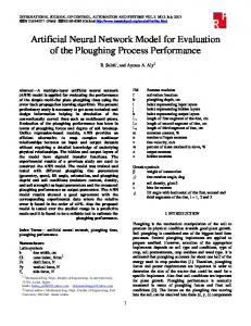
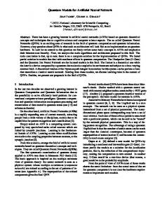
Neural Network (WNN) for forecasting by using the Trend and Threshold Autoregressive (T-TAR) model and it is applied to a nonstationary nonlinear time series. The analysis results were compared with that of existing methods and shows that the Wavelet Neural Networks provide the best model for analyzing the nonstationary nonlinear time series. Gonzalez-Concepcion, et al. (2010) used wavelets to reveal the different cycles that are hidden by the data. So, they consider some of the advantages and drawbacks of the time series multiresolution analysis technique for the purpose of obtaining simultaneous time and frequency information in determining the periodicity and the modelling of the water, energy and electricity consumption. The overall objective of this research is to develop an accurate model to forecast short and long term municipal water demand and apply it to the available data of water consumption. In order to meet this goal, a hybrid wavelet multilayer perceptron neural network model (Wavelet-ANN) has been developed. The model uses one dimensional discrete wavelet transforms to decompose the time series of water consumption data into its components which are modeled and forecasted individually by the multilayer perceptron neural network (MLP) then added together to produce the fitted series. The model applied to the time series of daily and monthly water consumption of Tampa city, USA. The study area and available data The data sources critical to the development of a comprehensive short and long water demand forecasting model include information from the economic, social, environmental, and water utility sectors. Because the development of the water forecasting model is dependent on the availability of water consumption data, therefore, to illustrate the applicability and capability of the model developed in the present study is applied to area, which can access to the required data. The area that the required data have been obtained for and the developed model applied to it as a case study is Tampa in the USA. The available data includes the daily water consumption and climatological data (minimum and maximum temperature, rainfall, mean relative humidity and mean wind speed) for a period of thirteen years from 1-January-1992 to 31December-2004 and the monthly data were derived from the daily data. The Tampa Bay Area is the region of west central Florida adjacent to Tampa Bay, USA. Tampa Bay Water is a regional wholesale drinking water utility that serves customers in the Tampa Bay, Florida region, USA as shown in Figure-1. The agency is special districts of the state created by inter local agreement among six member governments. Customers served in the area are predominantly residential users, with commercial, industrial and public consumption included (Asefa and Adams, 2007).

1048


ISSN 1819-6608



Figure-1. Tampa bay area map which is used as a study area in the research (Asefa and Adams, 2007). Model performance and accuracy measurements The most important criterion for evaluating forecasting models or choosing between competing models is accuracy. Generally speaking, the closer the forecasts to the observed values y, of the series, the more accurate the forecasting model is. Thus the quality of a model can be evaluated by examining the series of forecast errors ( ). The most commonly used measures of forecast accuracy are mean absolute error (MAE), mean squared error (MSE), root mean squared error (RMSE) and mean absolute percentage error (MAPE) (Rumantir, 1995). In addition to these measures, the most commonly used error measures in water resources modeling include the mean squared relative error (MSRE), the coefficient of determination (R2) and the coefficient of efficiency (CE) (Kingston, 2006). A more realistic way of assessing a model’s accuracy is to use a holdout set, that is, some of the data at the end of the series are omitted before the models are estimated. Then the models are compared on the basis of how well they forecast the data, which have been withheld rather than how well they forecast the same data which has been used for modeling (Makridakis, et al., 1998).

Therefore, in the present research for the purpose of selecting and comparison of forecasting models, the time series data were split into two sets. The first set of the data is used to estimate the parameters of the particular model (estimate set). Then with these estimates, the model is used to forecast ahead the remaining data points (holdout set). To obtain information about the model’s ahead forecasting performance; the resulting out of sample forecasts is compared to the actual holdout series values. Some of the above measures are used for holdout data and the model that yields best values for these statistics on holdout set would be chosen as a good model. For monthly water consumption data, the last 24 months of the data were to be held out, and then the model were fitted on the remaining data and used to forecast 24 months ahead. On the other hand, for daily water consumption data the last 5, 10 and 15 days of the data were held out. According to this partitioning of data, the number of estimation and holdout sets for the data considered in this research will be as shown in Table-1.

1049


ISSN 1819-6608



Table-1. Duration and estimation with holdout data sets for Tampa area. Data

Years

Duration

Estimation data no.

Holdout data no.

Monthly data

1992 - 2004

156 months

132

24

Daily data

1992 - 2004

4745 days

4740, 4735, 4730

5, 10, 15

The performance of the developed model in the present research were evaluated using some of the mentioned statistical measurements above that describe the errors associated with the model for estimating and holdout sets. In order to provide an indication of goodness of fit between the observed and each of predicted values for estimating set (fit) and holdout set (forecast), R2, RMSE and MAPE were used for the model investigated in this research as shown in the following equations:

In which N is the number of data points, are the observed data with its mean, respectively and , are the corresponding predicted data with its mean, respectively. Also two additional statistical tests, t-test and F-test were used in this research to compare the mean and variance of observed and predicted series for estimating and holdout sets. Among the most frequently used t-tests are a two sample location test of the null hypothesis that the means of two normally distributed populations are equal. The t-test statistic is:

Where N1 and N2 are the sub series sizes, Xi is the sample values in the N1 series and Xj in the N2 series. The variable t of Equation (4) follows the Student -distribution with (N1 + N2 – 2) degrees of freedom. The critical value tc for the 95% significance probability level is taken from the , then there is a difference in Student t-tables. If the mean of two series. In statistics, an F-test for the null hypothesis that two normal populations have the same variance is sometimes used. The expected values for two populations

can be different, and the hypothesis to be tested is that the variances are equal. The F-test statistic is:

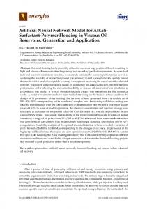
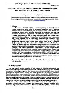
are the variances of observed and predicted Where , data, respectively. The observed and predicted sets have an F-distribution with N-2 degrees of freedom if the null hypothesis of equality of variances is true. The null hypothesis is rejected if F is either too large or too small. Multilayer perceptron neural network (MLP) The basic architecture of artificial neural network consists of three types of neuron layers: input layer, hidden layers and an output layer. Artificial neurons in one layer are connected, fully or partially, to the artificial neurons in the next layer. Feedback connections to previous layers are also possible (Engel brecht, 2007). A multilayer perceptron is feed forward neural network architecture with unidirectional full connections between successive layers. Figure-2 shows the structure of a multilayer perceptron artificial neural network which has an input layer, a hidden layer, and an output layer of neurons. These three layers are linked by connections whose strength is called weight. Thus there are two sets of weights: the input-hidden layer weights and the hiddenoutput layer weights. These weights provide the network with tremendous flexibility to freely adapt to the data; they are the free parameters, and their number is equivalent to the degrees of freedom of a network (Samarasinghe, 2006). The output of typical MLP neural networks with a single layer of hidden neurons, as shown in Figure-2, is given by:

is the output, n is the Where x is the input variable, number of neurons in input layer which is equal to the number of input variables, m is the number of neurons in hidden layer, w is the weights of input-hidden and hiddenoutput layers, b is the bias of hidden and output layers, fh is the activation function of hidden layer and fo is the activation function of output layer (Dreyfus, 2005). Training of multilayer perceptron artificial neural network basically involves feeding training samples as input vectors through a neural network, calculating the

1050


ISSN 1819-6608


www.arpnjournals.com error of the output layer, and then adjusting the weights of the network to minimize the error. The average of all the squared errors E for the outputs is computed to make the derivative easier. Once the error is computed, the weights can be updated one by one (Engel brecht, 2007). The sum of squares error is simply given by the sum of differences between the target and prediction outputs defined over the entire training set. Thus:

Input layer

Hidden layer

Where n is the number of training cases. It is clear that the bigger the difference between predictions of network and targets, the higher the error value, which means more weight adjustment, is needed by the training algorithm (Hill and Lewicki, 2007).

Output layer

x1

bj n

sj = wj,ixi+bj

xi

f h (sj)

f

hj

i=1

Bias x1

b

x1

b xn f1

x1 x1

1

bk m

1

f

sk = wk,jf h j+bk f o (sk)

j

yˆ k

j=1

f

xi

i

xn

n

j

wj,i w*j,i

m

Adjusted weights

k

m

yˆ Output

wk,j

Compare

y Target

Error

w*k,j

Back propagation training

Figure-2. Structure of typical multilayer perceptron artificial neural network. There are three main types of learning: supervised, unsupervised and reinforcement learning. The primary interests are the supervised learning algorithms, the most frequently used in real applications, such as the back propagation training algorithm, also known as the generalized delta rule. Two types of supervised learning algorithms exist based on when weights are updated:

Stochastic/online learning, where weights are adjusted after each pattern presentation. In this case the next input pattern is selected randomly from the training set, to prevent any bias that may occur due to the order in which patterns occur in the training set. Batch/offline learning, where weight changes are accumulated and used to adjust weights only after all training patterns have been presented.

Learning iterations which are referred to as epochs, consists of two phases: a) Feed forward pass, which simply calculates the output value(s) of the neural network for each training pattern. b) Backward propagation, which propagates an error signal back from the output layer toward the input layer. Weights are adjusted as functions of the back propagated error signal (Engel brecht, 2007).

It has been proven that back propagation learning with sufficient hidden layers can approximate any nonlinear function to arbitrary accuracy. This makes back propagation learning neural network a good candidate for signal prediction and system modeling (Abraham, 2005). The performance of neural networks is measured by how well they can predict unseen data (an unseen data set is one that was not used during training). This is known as generalization. There is a relation between over fitting the training data and poor generalization (Hill and Lewicki, 2007). That is, neural networks that over fit cannot predict correct output for data patterns not seen during training. Therefore, generalization is a very important aspect of neural network learning (Engel brecht, 2007). To avoid over fitting, the flexibility of a neural network must be reduced. Flexibility comes from the hidden neurons and as the number of hidden neurons increases, the number of network parameters (weights) increases as well. On the other hand, there must be enough neurons to avoid bias or under fitting (Samarasinghe, 2006). There are several techniques to combat the problem of over fitting and tackling the generalization issue. The most popular is cross validation which is a traditional statistical procedure for random partitioning of collected data into a training set and a test set (Palit and Popovic, 2005). Test data is a holdout sample that will never be used in training. Instead, it will be used to halt training to

1051


ISSN 1819-6608


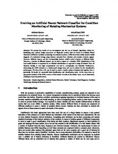
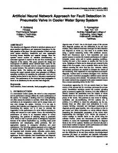
www.arpnjournals.com mitigate over fitting. The process of halting neural network training to prevent over fitting and improving the generalization ability is known as early stopping. Sometimes the test data alone may not be sufficient proof of a good generalization ability of a trained neural network. For example, a good performance on the test sample may actually be just a coincidence. To make sure that this is not the case, another set of data known as the validation sample is often used. Just like the test sample, a validation sample is never used for training the neural network. Instead, it is used at the end of training as an extra check on the performance of the model. If the performance of the network was found to be consistently good on both the test and validation samples, then it is reasonable to assume that the network generalizes well on unseen data. There are a number of main steps in the artificial neural network development process as shown in Figure-3 and there are also a number of options available at each step and, while this provides great flexibility in artificial neural network modeling, it also leaves the modeler faced with the difficult task of selecting the most suitable methods. One of the most important steps in using a neural network to solve real world problems is to collect and transform data into a form acceptable to the neural network. In practice, the simplest and linear transformation are most frequently used and obtained by rescaling or by standardization as follows:

, and maximum of untransformed data and are the mean and standard deviation of untransformed data (Palit and Popovic, 2005). In this section the focus will be on MLP neural network, which is the most popular and widely used network pattern in many applications including forecasting. For an explanatory or causal forecasting problem, the inputs to an ANN are usually the independent or predictor variables. The functional relationship estimated by the ANN can be written as:

Where are s independent variables and is a dependent variable. In this sense, the neural network is functionally equivalent to a nonlinear regression model. On the other hand, for an extrapolative or time series forecasting problem, the inputs are typically the past observations of the data series and the output is the future value. The ANN performs the following function mapping:

Where is the observation at time t. Thus the ANN is equivalent to the nonlinear autoregressive model for time series forecasting problems. It is also easy to incorporate both predictor variables and time lagged observations into one ANN model, which amounts to the general transfer function model (Zhang, et al., 1998). In order to complete the combination of Wavelet and ANN in the next sections, the components produced by the wavelet transform were modeled as a time series by using MLP neural network.

is the untransformed data, is the Where transformed data, , are the minimum

1052


ISSN 1819-6608



Figure-3. Main steps in the development of an artificial neural network (Kingston, 2006). Discrete wavelet transform (DWT) The wavelet is manipulated in two ways: the first one is translation in which the central position of the wavelet is changed along the time axis. The second one is scaling in which the transform is computed at various locations of the signal and for various scales of the wavelet, thus filling up the transform plane. If the process is done in a smooth and continuous fashion (i.e., if scale and position are varied very smoothly) then the transform is called continuous wavelet transform. If the scale and position are changed in discrete steps, the transform is called discrete wavelet transform (Soman, et al., 2011). The most basic wavelet transform is the Haar transform described by Alfred Haar in 1910. It serves as the prototypical wavelet transform. In 1988, Daubechies constructed a family of easily implemented and easily

invertible wavelet transforms that, in a sense, generalize the Haar transform (Selesnick, 2007). In today's world, computers are used to do almost all computations. It is apparent that neither the Fourier transform, nor the short time Fourier transform, nor the continuous wavelet transform can be practically computed by using analytical equations, integrals, etc. (Radunovic, 2009). As a matter of fact, the wavelet series is simply a sampled version of the continuous wavelet transform, and the information it provides is highly redundant as far as the reconstruction of the signal is concerned. This redundancy, on the other hand, requires a significant amount of computation time and resources. The discrete wavelet transform (DWT), on the other hand, provides sufficient information both for analysis and synthesis of

1053


ISSN 1819-6608


www.arpnjournals.com the original signal, with a significant reduction in the computation time (Mahmood, 2008). Discrete wavelets are usually part by part continuous functions and cannot be scaled and translated continuously, but only in discrete steps:

Where j and k are integers, while ao > 1 is the fixed scaling step. It is usually chosen to be ao = 2, so that the division on the frequency axis is dyadic. The translation factor is usually chosen to be bo = 1, so that the division on the time axis of the selected scale is uniform:

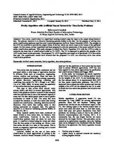
When the scaling parameter a is discretized on the logarithmic scale, the time parameter b is discretized depending on the scaling parameter, i.e., a different number of points is used at various scales. Using discrete wavelets, obtained by discretizing the scaling and translation parameters, is not discrete wavelet transform. The coefficients are still determined by the integrals, and the function f (t) is represented by a series, as a sum of the matching wavelets multiplied by the coefficients. To derive the discrete wavelet transformation it has to discretize the algorithm for calculating wavelet coefficients (Radunovic, 2009). Wavelet analysis is usually about approximations and details. Approximations are low frequency components of a function at large scale, while details are high frequency components of a function at smaller scales. The time scale representation of a signal is obtained using filtering techniques. In discrete wavelet transform, filters of different cutoff frequencies are used to analyze the signal at different scales. The signal is passed through a series of high pass filters to analyze the high frequencies, and it is passed through a series of low pass filters to analyze the low frequencies (Daubechies, 1992). The discrete wavelet transform analyzes the signal at different frequency bands with different resolutions by decomposing the signal into a coarse approximation and detail information. This transform employs two sets of functions, called scaling functions and wavelet functions, which are associated with low pass and high pass filters, respectively. The decomposition of the signal into different frequency bands is simply obtained by successive high pass and low pass filtering of the time domain signal. The original signal x[n] is first passed through a half band high pass filter g[n] and a low pass filter h[n]. After the filtering, half of the samples can be eliminated according to the Nyquist’s rule. The signal can therefore be subsampled by two, simply by discarding every other sample (Chui, 1997). This constitutes one

level of decomposition and can mathematically be expressed as follows:

Where yhigh [k] and ylow [k] are the outputs of the high pass and low pass filters, respectively, after sub sampling by 2 (Daubechies and Sweldens, 1998). This decomposition halves the time resolution since only half the number of samples now characterizes the entire signal. However, this operation doubles the frequency resolution, since the frequency band of the signal now spans only half the previous frequency band, effectively reducing the uncertainty in the frequency by half. The above procedure, which is also known as the sub band coding, can be repeated for further decomposition. At every level, the filtering and sub sampling will result in half the number of samples (and hence half the time resolution) and half the frequency band spanned (and hence doubles the frequency resolution). The high pass and low pass filters are not independent of each other, and they are related by: Where L is the filter length (in number of points). The reconstruction in this case is very easy since half band filters form orthonormal bases. The above procedure is followed in reverse order for the reconstruction. The signals at every level are up sampled by two, passed through the synthesis filters g[n] and h[n] (high pass and low pass, respectively), and then added. The interesting point here is that the analysis and synthesis filters are identical to each other, except for a time reversal. Therefore, the reconstruction formula for each layer becomes:

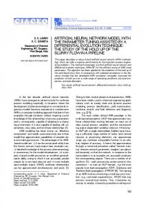
However, if the filters are not ideal half band, then perfect reconstruction cannot be achieved. Although it is not possible to realize ideal filters, under certain conditions it is possible to find filters that provide perfect reconstruction. The most famous ones are the ones developed by Ingrid Daubechies, and they are known as Daubechies’ wavelets (Mahmood, 2008). Figure-4 illustrates a two level decomposition of the original signal x[n] into approximations by passing through low pass filters h[n] and high pass filters g[n] then reconstructing the signal by up sampling. In wavelet analysis, a signal is split into an approximation and a detail. The approximation is then itself split into a second level approximation and detail, and the process is repeated. For a j-level decomposition, there are j+1 possible ways to decompose or encode the signal x[n] as follow (Nason, 2008):

1054


ISSN 1819-6608


www.arpnjournals.com g[n]

g'[n] n/2

2

n/2

D1[n]

g[n] 2

x[n]

2

n/4

D2[n]

n/4

2

A1[n]

x[n]

2

h[n] 2

n/4

h'[n]

A2[n]

h[n]

Analysis Decomposition

2

g'[n]

2

n/4 h'[n]

Coefficients, Details and Approximations

Synthesis Reconstruction

Figure-4. Decomposition and reconstruction of discrete wavelet transform (Misiti, et al., 2010). One of the most important achievements in wavelet theory was the construction of orthogonal wavelets that were compactly supported but were smoother than Haar wavelets. Wavelets with compact support have many interesting properties. They can be constructed to have a given number of derivatives and to have a given number of vanishing moments (Debnath, 2002). Daubechies in 1988 constructed such wavelets by an ingenious solution of the scaling function that resulted in a family of orthonormal wavelets (several families actually). Each member of each family is indexed by a number N, which refers to the number of vanishing moments (Nason, 2008). The Daubechies wavelets have no explicit expression except for db1, which is the Haarwavelet, which wavelet function resembles a step function (Merry, 2005). The Daubechies wavelet transform is implemented as a succession of decompositions. For example, the Daubechiesdb2 transform has four wavelet and scaling function coefficients. The scaling function coefficients for normalized are:

smoothed values are stored in the lower half of the n element input vector. On the other hand, the wavelet function will be applied to calculate n/2 differences (reflecting change in the data) and the wavelet values are stored in the upper half of the n element input vector. The scaling and wavelet functions are calculated by taking the inner product of the coefficients and four data values. For the simplest of the Daubechies wavelet transforms db2, the decomposition is given by:

The inverse block that reverses this decomposition uses the same coefficients and is given by (Selesnick, 2007):

The index iis incremented by two with each iteration, and new scaling and wavelet function values are calculated. Once the coefficients are obtained, the wavelet function coefficients can be found by reversing the coefficients and change the sign at the alternate positions (Soman, et al., 2011):

Each step of the wavelet transform applies the scaling and wavelet functions to the data input. If the original data set has n values, the scaling function will be applied in the wavelet transform step to calculate n/2 smoothed values. In the ordered wavelet transform the

Hybrid wavelet neural network The wavelet technique allows decomposing an original signal into several components in multiple scales. In wavelets, a low pass and a high pass filter are applied, extracting the low (approximations) and high (details) frequencies of the signal for the level of decomposition chosen, whose sum is equal to the original series; and which becomes smoother as the level increases. The idea when applying hybrid discrete wavelet transforms artificial neural network for time series analysis and forecasting is to decompose the original time series signal into smoother components and then to apply the most appropriate ANN prediction model for each component, individually. In this context, the low frequency components contain the general tendencies of

1055


ISSN 1819-6608


www.arpnjournals.com the series and can be used to explain the long term trend, while the high frequency components are best to explain near future trends. Time series of monthly municipal water consumption may have a historical pattern of variation that can be separated into long-memory components and shortrun components. Long-memory components are a trend which reflects the year to year effect of slow changes in population, water price, and family income; and seasonality which reflects the cyclic pattern of variation in water use within a year. Short-term components could be autocorrelation which reflects linear dependence of successive water consumption amounts and climate correlation which reflects the effect on water consumption of abnormal climatic events such as no rainfall or a lot of rainfall. In the model developed in this research, the one dimensional discrete wavelet transforms were applied, using the Daubechies function of order 1 to 5 with a resolution level of 1 to 5 for each order. The original water consumption data series was initially decomposed on its approximation and details. The components (approximation and details) were then modeled using the traditional MLP neural network as individual time series and then the predictive results obtained for each component were added to build the final results of the model. Multiresolution decomposition of time series The present research focuses on the multiresolution decomposition of a discrete signal for the daily and monthly water consumption data of Tampa.

Rewriting the Equation (20), the multiresolution decomposition of the variable or signal y[n] for al-level decomposition will be as follows:

Where A and D are the approximation and details of the signal decomposition respectively. The approximation Al is called the trend signal and Dl is the detail signal at level l constructed using the scaling function, representing the low frequency and high frequency wavelets, respectively. The original signal can be forecasted using wavelet decomposing arithmetic if D1, D2, …, Dl and Al can be forecasted. Water consumption fluctuates with time, so the fluctuation speed is different if the time is different. That means it has the characteristic of different frequency, either high or low. The fluctuation characteristic of the water consumption can be got through wavelet transform characteristics, and it should be transformed many times to get the fluctuation characteristic when the precision is dissatisfied. The interpretation of the multiresolution decomposition using the discrete wavelet transforms and its inverse is of interest in terms of understanding the frequency at which activity in the time series occurs. In our case, with daily and monthly water consumption time series, the interpretation of the different scale Dl with a dyadic dilation is given in Table-2.

Table-2. Interpretation of the different scale Dj for daily and monthly time series. Scale

Daily frequency resolution between

Monthly frequency resolution between

D1

2-4 days

2-4 months (including quarterly cycle)

D2

4-8 days (including weekly cycle)

4-8 months (including bi-annual cycle)

D3

8-16 days (including bi-weekly cycle)

8-16 months (including annual cycle)

D4

16-32 days (including monthly cycle)

16-32 months

D5

32-64 days (including bi-monthly cycle)

32-64 months

Wavelet reconstruction and forecasting The wavelet arithmetic was used to decompose water consumption time series using the Daubechies function and analyze its characteristics, i.e., to decompose the original time series into low frequency (approximation) A and high frequency (detail) D. The number of decomposed levels is decided by the minimal forecast error. When a time series of N data points is decomposed into l levels, then we get l+1 time series with N data points in each level. Traditional MLP neural networks were built to forecast the approximation and detail time series (decomposed time series). The final forecast value of the original water consumption can only be gained by synthesizing the forecast value of the artificial neural network models for all decomposed time series. The method to reconstruct the forecasted wavelet is

as in Equation (27). Figure-5 illustrates the flow chart of hybrid wavelet artificial neural network model. The approximation A and details D time series can be modeled by a neural network to discover nonlinear relationships in them. The artificial neural network models for the approximation and details with n past values as inputs are:

Where and are the nonlinear network model predictions of the approximation and details, represented by f, which is the function to be approximated by the neural network, and is the random error.

1056


ISSN 1819-6608



Figure-5. Flow chart of hybrid wavelet artificial neural network model. In the present research, traditional MLP architecture neural network will be introduced to process the wavelet approximation and details. The MLP architecture that is used for approximation and details time series prediction consists of one hidden layer with n neurons in the input layer, m neurons in the hidden layer and one output. The output of the multilayer perceptron MLP model for the approximation A and details D time series of l level discrete wavelet decomposition, with input nodes will be:

research for carrying out each step of the MLP neural network development processes are summarized in the followings: Neural network architecture: for forecasting the components produced by wavelet transform, a number of trials on several lags of the component series were made in order to correctly select the important inputs to the ANN. At the end, in this research a twelve lags of component will be used as input variables. There is only one output node for the neural network which is the component value at time t. A single hidden layer will be used in the neural networks. The trial and error way were used in determining the number of hidden nodes. Activation function: in this research, the tangent hyperbolic activation function was used in the hidden layer and linear function in the output layer for MLP networks developed for the components produced by wavelet transform.

Where

and

are the input variables,

and

are the outputs, is the number of neurons in input layer, which is equal to the number of input variables (approximation or detail time lags), m is the number of neurons in the hidden layer, w is the weights of inputhidden and hidden-output layers, , are the bias of hidden and output layers respectively, fh is the activation function of the hidden layer and fo is the activation function of the output layer. Following the designing artificial neural network steps given in Figure-3, the methods adopted in this

Data preprocessing: in this research, the input and target variables were preprocessed by using linear transformations such that the original minimum and maximum of every variable, are mapped to the range (-1, +1). Training and test sets: As mentioned earlier, the data set is usually divided into three subsets: training, test and validation subsets for building an ANN forecaster. The literature offers little guidance in selecting the training and the test sample. Most investigators select them based on the rule of 90% vs. 10%, 80% vs. 20% or 70% vs. 30%, etc. Some choose them based on their particular problems (Zhang, et al., 1998). In this study, as mentioned earlier, the entire available data set will be divided into estimate

1057


ISSN 1819-6608


www.arpnjournals.com and holdout subsets. The estimate subset was divided into training and test samples randomly for using in ANN modeling. The estimating sets of data were divided with 80% of the data allocated to training subset and 20% allocated to testing subset.

using the coefficient of determination (R2), the root mean squared error (RMSE) and the mean absolute percentage error (MAPE). In addition, the t-test and F-test were carried out for observed and forecasted data of time series in both cases.

Performance criteria: the ultimate and the most important measure of performance of ANNs model is the accuracy of forecasting that achieve beyond the training data. However, a suitable measure of accuracy for a given problem is not universally accepted by the forecasting academicians and practitioners. The commonly performance criteria, mentioned earlier will all be used to evaluate the performance of the trained MLPs developed for components produced by wavelet transform in this research, based on the fit and forecast data results. To perform the decomposition process for daily and monthly water consumption time series and building traditional MLP predicting models for approximation and details time series, a MATLAB code has been written called WAVELET-ANN. The WAVELET-ANN code has been written using MATLAB version 7.0 package software to combine the one dimensional discrete wavelet transforms with MLP neural network processes. The code performs preprocessing and decomposition of the time series into approximation and details, then using MLP neural networks for training and forecasting of decomposed time series. Finally, the predicted values of approximation and details are added together to form the predicted values of the original time series. The code consists of a main program and three subprograms for creating, retraining and forecasting MLP models.

Monthly water consumption time series As stated before, the developed Wavelet-ANN model has been applied to monthly water consumption time series of Tampa, USA. The time series were divided into two subsets: estimate subset for fitting the model and holdout subset at the end of the series (last 24 months) for evaluating the forecasting ability of the model. For the time series, twenty five models were developed using the Daubechies function of order ranging from 1 to 5 and multiresolution level ranging from 1 to 5 for each order of the function (dbilj, i=1, 2,…, 5 and j=1, 2, …, 5). In which db refers to the Daubechies function, i is the order of the function, l is the resolution and j is the level of the resolution. For a model with j resolution levels there are j+1 decomposed time series (approximation and details) that can be predicted by modeling using the traditional MLP neural network. As mentioned earlier, the time series will be scaled linearly into the range (-1, +1) before decomposition by discrete wavelet transforms. The input variables to the MLP models for the approximation and details time series are the past values of the decomposed time series. For monthly water consumption decomposed time series, the lagged values (At-1, At-2, …, At-12) and (Dt-1, Dt-2, …, Dt-12) were used as input variables to the input neurons of the input layer of each MLP model for approximation and details time series respectively. In the MLP models, only one hidden layer and one output layer consisting of one node denoting the predicted value were used. The trial-and-error procedure was used to select the optimum number of hidden neurons in the hidden layer. Furthermore, only the tangent hyperbolic and linear activation functions have been used in the hidden and output layers respectively. All MLP models for approximation and details series were trained using the back propagation algorithm. The data in the estimate set of data were partitioned randomly into 80% as training samples and 20% as testing samples. First, the decomposition of the time series (approximation and details) for monthly water consumption time series would be carried out, then the MLP models for each approximation and details time series were trained using the data in the estimate subset to obtain the optimized set of connection strengths (weights). The predicted values for the model were obtained by summing the predicted values of the MLP models for decomposed time series (approximation and details). In the forecasting phase, after training the MLP neural networks, they are used to predict sub time series (approximation and details) with a specific lead time (holdout subset). The forecasted time series can then be reconstructed by inverting the discrete wavelet transforms. The model is then evaluated using the data in the holdout

The model application Decomposing the original time series using the discrete wavelet transforms produces many sub time series. Depending on the depth of the analysis, these sub time series highlight the trends and the periodicity that exist in the original time series. Wavelet decomposition can be used to produce a large number of sub time series. Therefore, the decomposition is truncated and only few sub time series are used. The used sub time series are chosen in a way that preserves the information from the time series. Each sub time series obtained from the multiresolution analysis can be modeled using MLP models. To demonstrate the forecasting capability of the developed Wavelet-ANN model, two cases are considered, one for monthly water consumption and the other for daily water consumption. The model has been applied to daily and monthly municipal water consumption time series of Tampa, USA. As mentioned earlier, the ANN models developed for decomposed time series (approximation and details) were the traditional MLP neural network with three layers, and the activation functions of the hidden and output layers were fixed to tangent hyperbolic and linear respectively. For each daily and monthly water demand forecasting problem, the performance of the developed Wavelet-ANN models has been measured and compared

1058


ISSN 1819-6608


www.arpnjournals.com subset and compared using the statistical measures of goodness of fit. The statistical performance measurements of the results for monthly water consumption time series for estimate and holdout sets of Tampa are shown in Table-3. Comparing the results of the developed models for monthly water consumption time series, generally, the performance of Wavelet-ANN model for the estimate set of data increases by increasing the order of the Daubechies function. On the other hand, for holdout set of data, it is clear that the best results are obtained by using the 4th order of Daubechies function for the problem considered in this study. Note that the required resolution level to obtain the best results depends on the characteristics of the time series. For monthly water consumption time series considered in this study, in general, the Wavelet-ANN models with the higher order of Daubechies function are performing better than the models with lower order function for each of the estimate and holdout set of data. It is clear from the results, that using the low order Daubechies function requires more decomposition levels to obtain best results, and this is because the low order function is less smooth than the high order function. Most of the models with 3-5 order of Daubechies function have the best results in the range of 2-5 of decomposition level and this is due to the relative high presence of random component in the monthly water consumption time series of Tampa. Comparing the statistical measurements of the developed models, for the estimate set of data, model M24 (db5l4) has the best performance with the highest value of R2 (0.990) and lowest values of MAPE (0.984%) and RMSE (230259). On the other hand, for the holdout set of data, model M17 (db4l2) has the best performance with the highest value of R2 (0.982) and lowest values of MAPE (0.812%) and second lowest values of RMSE (197819). Comparing the t-test and F-test values for all models of monthly data considered in this study with corresponded critical t and F values indicate that the hypotheses are not statistically significant. The observed and forecasted values of the two best models for each monthly water consumption time series for estimate and holdout sets are shown in Figure-6. Daily water consumption time series The second case in which Wavelet-ANN model was applied is short term forecasting of daily water consumption time series of Tampa. As mentioned in this study, the daily water consumption series in Tampa is from 1st January, 1992 to 31st December, 2004 (4745 observations). The 29th days of February in the leap years have been dropped from the series in order to maintain 365 days in each year. The first 4740, 4735 and 4730 observations from 1st January, 1992 were used as training samples for model estimation, and the remaining 5, 10 and 15 observations were used as a holdout samples for forecast evaluation respectively. Three types of WaveletANN models for the daily data were developed: 5, 10 and

15 days ahead forecasting models. For each type, twenty five models were developed using the Daubechies function of order ranges from 1 to 5 and decomposition level ranging from 1 to 5 for each order of the function (dbilj, i =1, 2,…, 5 and j =1, 2, …, 5). As for monthly data, the time series was scaled linearly into the range (-1, +1) before the decomposition process. The input variables to the MLP models for the approximation and details time series were the past values of the decomposed time series. The time lagged values (At1, At-2, …, At-7) and (Dt-1, Dt-2, …, Dt-7) were used as input variables to the input neurons of the input layer of each MLP model for approximation and details time series respectively. The MLP neural network models of decomposed series consist of one hidden layer and one neuron in the output layer. The number of neurons in the hidden layers of MLP models was determined by trial and error. All MLP models for approximation and details series were trained using the back propagation algorithm. The data in the estimate set of data were partitioned randomly into 80% as a training sample and 20% as a testing sample. Furthermore, only the tangent hyperbolic and linear activation functions have been used in the hidden and output layers, respectively. After applying the Wavelet-ANN models to forecast daily urban water demand by the area of Tampa in the USA, the performances of the models were evaluated using R2, MAPE and RMSE statistics for estimate and holdout sets. The statistical performance measurements of the results of daily water demand forecasting of Tampa for the estimate and holdout sets of 5, 10 and 15 days ahead forecasting models are shown in Tables 4 through 6, respectively. Generally, comparing the results of the developed models for the estimate and holdout set of data; it can be observed that the models with a higher decomposition level and higher order of the Daubechies function perform better than those with a lower decomposition level and functions of lower order. This is due to the presence of periodicity, randomness and other irregular components in the daily series that cannot be separated by decomposition of low levels. As it is clear from the results, for the estimate set of data of 5 and 10 days ahead forecasting models, model M23 (db5l3) with the Daubechies functions of 5th order and three levels of decomposition have the best performance with the highest R2 values and lowest MAPE and RMSE values, while for 15 days ahead forecasting model, model M25 (db5l5) has the best result. On the other hand, for holdout set of data of 5 days ahead forecasting models, model M19 (db4l4) has the 2nd highest value of R2 (0.991), the 2nd lowest value of MAPE (0.570%) and the 3rd lowest value of RMSE (4033). The highest value of R2 and the lowest values of MAPE and RMSE are distributed among the models M22 (db5l2), M25 (db5l5) and M15 (db3l5), respectively. For holdout set of data of 10 days ahead forecasting models, model M18 (db4l3) has the 2nd highest value of R2 (0.989) and the lowest values of MAPE (0.947%) and RMSE (6428). For holdout set of data of 15 days ahead forecasting

1059


ISSN 1819-6608


www.arpnjournals.com models, model M19 (db4l4) has the highest value of R2 (0.967) and the lowest values of MAPE (1.029%) and RMSE (8136). It can be observed from the results that the accuracy of forecasting decreases by increasing the forecasting periods ahead, and this is axiomatic. The application results show that the developed forecasting model seems to provide highly accurate daily forecasts for 5 days as well as for 10 and 15 days into the future.

Comparing the t-test and F-test values of all WaveletANN models for the three considered cases (5, 10 and 15 days ahead forecasting) with corresponded critical t and F values indicates that there are no differences in the mean and variance between the observed and forecasted series for in-sample (estimate) and out-sample (holdout) sets. The observed and forecasted values of the two best models for each case of daily water consumption time series of Tampa for estimate and holdout set are shown in Figure-7.

Table-3. Daubechiesfunction order, resolution level and statistical performance measurements of wavelet-ANN models of monthly water consumption time series for Tampa.

R2

MAPE (%)

RMSE

t-value

F-value

R2

MAPE (%)

RMSE

t-value

F-value

M1

Daubechies function order and resolution level db1l1

0.919

2.172

664512

0.028

1.100

0.668

3.197

793810

0.297

1.058

M2

db1l2

0.936

2.096

600986

0.203

1.135

0.687

2.795

794164

-0.251

1.082

M3

db1l3

0.915

2.224

682533

0.033

1.073

0.754

2.228

743763

-0.490

1.192

M4

db1l4

0.900

2.541

741308

0.080

1.088

0.727

2.376

745698

-0.424

1.061

M5

db1l5

0.910

2.249

702355

0.090

1.077

0.739

2.190

752186

-0.551

1.111

M6

db2l1

0.945

1.961

551993

0.011

1.092

0.898

2.171

464853

0.014

1.203

M7

db2l2

0.957

1.858

488132

0.030

1.107

0.880

1.937

466345

0.187

1.030

M8

db2l3

0.967

1.682

426245

-0.021

1.063

0.923

1.716

391003

0.309

1.029

M9

db2l4

0.957

2.012

488533

0.021

1.084

0.920

1.608

378236

0.119

1.001

M10

db2l5

0.958

1.901

480553

0.079

1.085

0.915

1.679

384401

-0.024

1.101

M11

db3l1

0.966

1.710

434845

0.029

1.008

0.881

1.940

483372

0.194

1.098

M12

db3l2

0.971

1.622

410724

-0.014

1.044

0.960

1.259

279905

-0.008

1.106

M13

db3l3

0.971

1.604

404628

-0.057

1.044

0.968

1.368

310482

0.045

1.291

M14

db3l4

0.975

1.452

380681

-0.047

1.049

0.974

1.230

254784

0.007

1.195

M15

db3l5

0.978

1.405

358338

-0.044

1.051

0.973

1.114

263641

0.030

1.209

M16

db4l1

0.968

1.604

424523

0.082

1.006

0.924

1.626

376648

-0.176

1.030

M17

db4l2

0.984

1.224

303758

0.005

1.025

0.982

0.812

197819

0.073

1.087

M18

db4l3

0.985

1.163

288449

0.014

1.033

0.982

0.953

220239

-0.083

1.183

M19

db4l4

0.986

1.152

281194

-0.008

1.025

0.982

0.873

203770

-0.023

1.144

M20

db4l5

0.986

1.187

284484

0.027

1.032

0.978

0.945

206007

-0.149

1.016

M21

db5l1

0.969

1.628

410632

0.048

1.027

0.937

1.519

336544

-0.134

1.124

M22

db5l2

0.988

1.031

254476

0.042

1.015

0.963

1.156

254947

-0.005

1.026

M23

db5l3

0.989

1.024

242992

0.041

1.011

0.980

0.849

197551

-0.156

1.026

M24

db5l4

0.990

0.948

230259

0.034

1.015

0.978

0.892

200072

-0.112

1.012

M25

db5l5

0.989

1.009

244017

0.001

1.005

0.978

0.883

205722

-0.070

1.060

2.256

1.435

2.317

2.312

Model

Estimate set (Observed - Fit)

Critical values of t and F

Holdout set (Observed - Forecast)


1060


ISSN 1819-6608


www.arpnjournals.com 3.00E+07 Holdout Set (Observed-Forecast)

Estimate Set (Observ ed-Fit)

2.80E+07

Water Consumption (m 3)

2.60E+07 2.40E+07 2.20E+07 2.00E+07 1.80E+07 1.60E+07

Fit

Forecast (M17-db4l2)

Fit

Jul-2004

Jul-2003

Jan-2004

Jul-2002

Jan-2003

Jul-2001

Jan-2002

Jul-2000

Jan-2001

Jul-1999

Jan-2000

Jul-1998

Jan-1999

Jul-1997

Jan-1998

Jul-1996

Jan-1997

Jul-1995

Jan-1996

Jul-1994

Observ ed

Jan-1995

Jul-1993

Jan-1994

Jul-1992

Jan-1993

1.20E+07

Jan-1992

1.40E+07

Forecast (M24-db5l4)

Figure-6. Observed, fit and forecast of wavelet-ANN models for monthly water consumption time series of Tampa. Table-4. Daubechies function’s order, resolution level and statistical performance measurements of wavelet-ANN models of daily water consumption time series for Tampa - forecasting 5 days ahead. Model M1 M2 M3 M4 M5 M6 M7 M8 M9 M10 M11 M12 M13 M14 M15 M16 M17 M18 M19 M20 M21 M22 M23 M24 M25

Daubechies function order and resolution level db1l1 db1l2 db1l3 db1l4 db1l5 db2l1 db2l2 db2l3 db2l4 db2l5 db3l1 db3l2 db3l3 db3l4 db3l5 db4l1 db4l2 db4l3 db4l4 db4l5 db5l1 db5l2 db5l3 db5l4 db5l5

Estimate set (Observed - Fit) R2

MAPE (%)


RMSE

t-value

F-value

0.863 2.177 20703 0.895 1.804 18106 0.906 1.769 17158 0.900 2.005 17725 0.902 1.964 17517 0.916 1.958 16125 0.951 1.503 12292 0.961 1.351 11071 0.964 1.339 10620 0.964 1.341 10619 0.941 1.733 13541 0.971 1.235 9569 0.977 1.094 8552 0.976 1.110 8609 0.975 1.124 8817 0.956 1.458 11682 0.979 1.062 8091 0.980 1.022 7840 0.981 0.988 7621 0.981 0.985 7612 0.961 1.456 10954 0.984 0.928 7054 0.986 0.887 6694 0.985 0.916 6917 0.986 0.887 6704 Critical values of t and F

0.013 -0.030 -0.029 -0.004 0.007 0.016 0.002 0.024 0.011 0.013 -0.003 0.005 0.005 0.004 0.005 -0.001 -0.012 -0.001 0.010 -0.018 -0.023 -0.012 -0.007 0.002 -0.001 2.242

1.224 1.173 1.161 1.184 1.179 1.104 1.055 1.049 1.067 1.057 1.051 1.011 1.011 1.008 1.013 1.032 1.015 1.011 1.014 1.014 1.037 1.008 1.009 1.013 1.009 1.059

R2

MAPE (%)

RMSE

t-value

F-value

0.805 1.939 15930 0.525 1.653 19389 0.500 2.236 20884 0.646 1.861 15178 0.583 1.921 16044 0.942 0.559 6823 0.833 1.318 10824 0.916 1.204 8495 0.981 0.826 6211 0.979 0.887 6130 0.802 1.545 11475 0.952 0.868 5619 0.978 0.736 5083 0.965 0.750 4992 0.985 0.598 3847 0.871 1.225 8998 0.948 0.948 7798 0.974 0.744 5267 0.991 0.570 4033 0.963 0.904 6530 0.969 1.386 9633 0.851 5979 0.996 0.966 0.636 4870 0.972 0.575 4170 0.976 3889 0.467 Critical values of t and F

0.672 0.507 0.470 0.092 0.060 0.156 0.120 0.064 -0.141 -0.098 0.033 0.055 -0.117 -0.090 -0.019 0.029 0.297 0.186 0.112 0.198 0.481 0.299 0.076 0.043 0.054 2.752

1.061 1.236 1.070 2.388 1.397 1.287 1.103 1.300 1.371 1.384 1.073 1.063 1.218 1.067 1.185 1.001 1.056 1.070 1.216 1.188 1.069 1.312 1.158 1.041 1.045 9.605

1061


ISSN 1819-6608


www.arpnjournals.com Table-5. Daubechies function’s order, resolution level and statistical performance measurements of wavelet-ANN models of daily water consumption time series for Tampa - forecasting 10 days ahead.

R2

MAPE (%)

RMSE

t-value

F-value

R2

MAPE (%)

RMSE

t-value

F-value

M1


0.865

2.130

20484

0.001

1.215

0.877

2.025

17803

0.063

1.480

M2

db1l2

0.894

1.834

18140

-0.016

1.170

0.592

3.914

31568

0.352

1.704

M3

db1l3

0.909

1.761

16882

-0.014

1.157

0.722

3.043

27689

0.513

1.671

M4

db1l4

0.904

1.935

17281

-0.021

1.164

0.779

2.902

23997

0.258

1.740

M5

db1l5

0.904

1.934

17333

-0.037

1.177

0.698

3.239

27399

0.311

1.695

M6

db2l1

0.916

1.978

16117

0.020

1.106

0.887

1.922

16935

-0.154

1.027

M7

db2l2

0.952

1.471

12149

0.017

1.058

0.938

1.264

12926

-0.154

1.079

M8

db2l3

0.961

1.345

10966

0.003

1.059

0.911

1.895

14716

-0.135

1.041

M9

db2l4

0.962

1.357

10830

-0.014

1.063

0.958

1.303

9974

-0.015

1.002

M10

db2l5

0.965

1.312

10461

0.007

1.061

0.928

1.838

15016

-0.245

1.147

M11

db3l1

0.940

1.762

13654

0.016

1.054

0.859

2.276

20790

-0.210

1.240

M12

db3l2

0.973

1.193

9123

0.025

1.012

0.966

1.474

12235

-0.247

1.226

M13

db3l3

0.974

1.151

8912

0.003

1.013

0.973

1.296

10018

-0.038

1.242

M14

db3l4

0.977

1.095

8496

0.019

1.012

0.969

1.596

11248

-0.136

1.255

M15

db3l5

0.978

1.068

8311

-0.001

1.011

0.986

1.121

8588

-0.086

1.255

M16

db4l1

0.959

1.421

11282

0.024

1.035

0.785

2.987

22584

-0.119

1.156

M17

db4l2

0.979

1.049

8051

-0.009

1.012

0.986

1.074

7576

0.121

1.223

M18

db4l3

0.981

0.982

7647

-0.008

1.011

0.989

0.947

6428

0.046

1.200

M19

db4l4

0.983

0.930

7194

-0.014

1.013

0.970

1.508

9665

0.003

1.279

M20

db4l5

0.981

0.991

7644

0.008

1.013

0.993

1.075

7873

0.120

1.328

M21

db5l1

0.963

1.431

10677

0.021

1.034

0.880

2.181

16766

0.088

1.170

M22

db5l2

0.984

0.932

7103

0.001

1.005

0.962

1.378

10871

0.090

1.314

M23

db5l3

0.986

0.878

6672

-0.002

1.006

0.980

1.146

9268

0.014

1.349

M24

db5l4

0.986

0.885

6677

-0.003

1.007

0.977

1.213

9483

0.029

1.336

M25

db5l5

0.985

0.893

6779

-0.003

1.005

0.981

1.168

9037

0.014

1.341

2.242

1.059

2.445

4.026

Model





1062


ISSN 1819-6608


www.arpnjournals.com Table-6. Daubechies function’s order, resolution level and statistical performance measurements of wavelet-ANN models of daily water consumption time series for Tampa - forecasting 15 days ahead.

R2

MAPE (%)

RMSE

t-value

F-value

R2

MAPE (%)

RMSE

t-value

F-value

M1


0.866

2.087

20458

-0.003

1.206

0.831

1.848

16663

-0.009

1.177

M2

db1l2

0.899

1.776

17794

-0.025

1.164

0.599

2.701

26046

0.308

1.751

M3

db1l3

0.909

1.800

16993

-0.011

1.179

0.676

2.470

23330

0.227

1.473

M4

db1l4

0.903

1.953

17508

0.009

1.179

0.736

2.455

21002

-0.031

1.581

M5

db1l5

0.904

1.941

17356

-0.007

1.180

0.751

2.308

20909

0.178

1.759

M6

db2l1

0.915

1.987

16269

0.007

1.096

0.867

1.641

15643

-0.140

1.093

M7

db2l2

0.953

1.432

12075

-0.017

1.054

0.918

1.230

12441

-0.093

1.130

M8

db2l3

0.958

1.452

11516

-0.011

1.055

0.937

1.462

11383

-0.083

1.183

M9

db2l4

0.968

1.263

10002

-0.015

1.055

0.898

1.531

13053

-0.048

1.035

M10

db2l5

0.967

1.285

10178

-0.021

1.060

0.890

1.615

13621

-0.062

1.032

M11

db3l1

0.941

1.732

13557

-0.006

1.056

0.826

2.086

17872

-0.111

1.085

M12

db3l2

0.972

1.226

9318

0.023

1.012

0.939

1.435

11951

-0.197

1.228

M13

db3l3

0.976

1.115

8645

0.005

1.010

0.955

1.431

10762

-0.100

1.280

M14

db3l4

0.977

1.087

8446

0.008

1.013

0.958

1.255

9855

-0.091

1.220

M15

db3l5

0.977

1.093

8515

0.009

1.013

0.964

1.318

9830

-0.162

1.249

M16

db4l1

0.958

1.470

11515

-0.013

1.031

0.751

2.449

20475

0.135

1.162

M17

db4l2

0.978

1.074

8250

0.006

1.018

0.953

1.364

9341

0.025

1.229

M18

db4l3

0.981

1.013

7787

0.005

1.015

0.958

1.125

8595

0.095

1.123

M19

db4l4

0.981

0.988

7678

-0.006

1.015

0.967

1.029

8136

0.012

1.233

M20

db4l5

0.981

0.990

7676

-0.008

1.017

0.960

1.148

8851

0.072

1.250

M21

db5l1

0.966

1.366

10364

0.007

1.039

0.873

1.912

14515

-0.044

1.093

M22

db5l2

0.985

0.909

6947

-0.004

1.002

0.951

1.197

9436

0.044

1.216

M23

db5l3

0.985

0.888

6733

-0.010

1.004

0.953

1.321

9749

0.044

1.304

M24

db5l4

0.985

0.888

6767

-0.009

1.006

0.958

1.285

9518

-0.018

1.332

M25

db5l5

0.986

0.888

6649

-0.004

1.008

0.961

1.275

9107

-0.016

1.312

2.242

1.059

2.368

2.979

Model





1063


ISSN 1819-6608


www.arpnjournals.com 7.00E+05 6.80E+05

Water Consumption (m 3)

6.60E+05 6.40E+05 6.20E+05 6.00E+05 5.80E+05 5.60E+05 5.40E+05 5.00E+05

Observ ed Fit Fit

1-Dec-04 2-Dec-04 3-Dec-04 4-Dec-04 5-Dec-04 6-Dec-04 7-Dec-04 8-Dec-04 9-Dec-04 10-Dec-04 11-Dec-04 12-Dec-04 13-Dec-04 14-Dec-04 15-Dec-04 16-Dec-04 17-Dec-04 18-Dec-04 19-Dec-04 20-Dec-04 21-Dec-04 22-Dec-04 23-Dec-04 24-Dec-04 25-Dec-04 26-Dec-04 27-Dec-04 28-Dec-04 29-Dec-04 30-Dec-04 31-Dec-04

5.20E+05

Fit Forecast (5 day s ahead f orecasting model M19-db4l4) Forecast (10 day s ahead f orecasting model M18-db4l3) Fit Forecast (15 day s ahead f orecasting model M19-db4l4) Fit

Fit Forecast (5 day s ahead f orecasting model M23-db5l3) Forecast (10 day s ahead f orecasting model M23-db5l3) Forecast (15 day s ahead f orecasting model M25-db5l5)

Figure-7. Observed, fit and forecast series of wavelet-ANN models for daily water consumption time series of Tampa. CONCLUSIONS The model developed in this research for daily and monthly municipal water demand forecasting is a hybrid Wavelet-ANN that combines the discrete wavelet transform (DWT) method with the multilayer perceptron artificial neural network model (MLP). The results obtained in this research are highly promising demonstrating the effectiveness of the Wavelet-ANN model in forecasting daily and monthly municipal water demand. It is quite clear from the results of the developed hybrid Wavelet-ANN time series model that the model provides accurate daily and monthly forecasts as measured using a validation period of 5, 10 and 15 for daily data and 24 months for monthly data.

Chui C. K. 1997. Wavelets: A Mathematical Tool for Signal Analysis. Philadelphia: Society for Industrial and Applied Mathematics, Siam. Daubechies I. 1992. Ten Lectures on Wavelets. Philadelohia, PA, Society for Industrial and Applied Mathematics. Daubechies I. and Sweldens W. 1998. Factoring Wavelet Transforms into Lifting Steps. Journal of Fourier Analysis and Applications. 4(3): 247-269. Debnath L. 2002. Wavelet Transforms and Their Applications. Boston: Birkhauser, Bertelsmann Springer Science+Business Media GmbH.

REFERENCES Abraham A. 2005. Artificial Neural Networks. In: Handbook of Measuring System Design. s.l. John Wiley and Sons, Ltd. pp. 901-908. Alaa H. A. and Nisai W. 2004. Short Term Forecasting for Urban Water Consumption. Journal of Water Resources Planning and Management, 1st September. 130(5): 405410. Asefa T. and Adams A. 2007. Short Term Urban Water Demand Forecast Models in Action: Challenges from Model Development to Implementation to Real Time Operations. Tampa, Florida, ASCE. Bougadis J., Adamowski K. and Diduch R. 2005. Short Term Municipal Water Demand Forecasting. Journal of Hydrological Processes, January. 19(1): 137-148.

Dreyfus G. 2005. Neural Networks: Methodology and Applications. 2nd Ed. s.l.: Springer-Verlag Berlin Heidelberg. Engelbrecht A. P. 2007. Computational Intelligence: An Introduction. 2nd Ed. The Atrium, Southern Gate, Chichester, West Sussex PO19 8SQ: John Wiley and Sons Ltd. Ghiassi M., Zimbra D. K. and Saidane H. 2008. Urban Water Demand Forecasting with a Dynamic Artificial Neural Network Model. Journal of Water Resources Planning and Management. 134(2): 138-146. Gonzalez-Concepcion C., Gil-Farina M. C. and PestanoGabino C. 2010. Wavelets Modelling of Water, Energy and Electricity Consumption in Spain. Journal of WSEAS TRANSACTIONS on MATHEMATICS. 9(7): 509-518.

1064


ISSN 1819-6608


www.arpnjournals.com Hill T. and Lewicki P. 2007. Statistics Methods and Applications. Tulsa, OK: StatSoft, Inc.

Nason G. P. 2008. Wavelet Methods in Statistics with R. New York: Springer Science+Business Media, LLC.

Jain D. A., Varshney A. K. and Joshi U. C. 2001. Short Term Water Demand Forecasting at IIT Kanpur Using Artificial Neural Networks. Journal of Water Resources Management, October. 15(5): 299-321.

Palit A. K. and Popovic D. 2005. Computational Intelligence in Time Series Forecasting, Theory and Engineering Applications. London: Springer-Verlag London Limited.

Kim J. H., Hwang S. H. and Shin H. S. 2001. A NeuroGenetic Approach for Daily Water Demand Forecasting. KSCE. Journal of Civil Engineering, September. 5(3): 281-288.

Radunovic D. P. 2009. WAVELETS from MATH to PRACTICE. Berlin Heidelberg: SPRINGER-VERLAG.

Kim T.-W. and Valdes J. B. 2003. Nonlinear Model for Drought Forecasting Based on a Conjunction of Wavelet Transforms and Neural Networks. Journal of Hydrologic Engineering, ASCE. 8(6): 319-328. Kingston G. B. 2006. Ph.D Thesis. Adelaide: Computer and Mathematical Sciences, Faculty of Engineering, School of Civil and Environmental Engineering, The University of Adelaide, Australia. Li S. 2002. Traffic Flow Prediction of Intersections Using Wavelet Neural Network. s.l., Applications of Advanced Technologies in Transportation. Proceedings of the 7th International Conference, ASCE. Mahmood S. A. 2008. Ph.D Thesis. Sulaimani(Kurdistan Region): College of Science, University of Sulaimani, Iraq. Makridakis S., Wheelwright S. C. and Hyndman R. J. 1998. Forecasting, Methods and Applications. 3rd Ed. New York: John Wiley and Sons, Inc.. Merry R. J. 2005. A literature study. Eindhoven: Control Systems Technology Group, Department of Mechanical Engineering, Eindhoven University of Technology. Minu K. K., Lineesh M. C. and John J. C. 2010. Wavelet Neural Networks for Nonlinear Time Series Analysis. Journal of Applied Mathematical Sciences. 4(50): 24852495. Misiti M., Misiti Y., Oppenheim G. and Poggi J.-M. 2010. Wavelet Toolbox™ User’s Guide. R2010b, MATLAB ed. s.l.:The MathWorks, Inc.. Msiza I. S., Nelwamondo F. V. and Marwala T. 2007. Artificial Neural Networks and Support Vector Machines for Water Demand Time Series Forecasting. Montreal, Quebec, Canada, IEEE. pp. 638-643.

Rumantir G. W. 1995. M.Sc Thesis. Melbourne: Department of Computer Science, Royal Melbourne Institute of Technology. Samarasinghe S. 2006. Nueral Networks for Applied Sciences and Engineering: From Fundamentals to Complex Pattern Recognition. New York: Taylor and Francis Group, LLC. Selesnick I. W. 2007. Wavelet Transforms: A Quick Study. Physics Today magazine, October. Soman K. P., Ramachandran K. I. and Resmi N. G. 2011. Insights In to Wavelets: From Theory to Practice. 3rd Ed. New Delhi: Eastern Economy Edition. Wei Y. X. and Liang X. R. 2007. Freeway Traffic Flow Modeling Based on Recurrent Neural Network and Wavelet Transform. s.l., International Conference on Transportation Engineering, Proceedings of the 1st International Conference, ASCE. Xie Y. and Zhang Y. 2006. Application of Wavelet Time Series Analysis in Short-Term Traffic Volume Prediction. s.l., Applications of Advanced Technology in Transportation. Proceedings of 9th International Conference, ASCE. Yurdusev M. A. and Firat M. 2009. Adaptive Neuro Fuzzy Inference System Approach for Municipal Water Consumption Modelling: An Application to Izmir, Turkey. Journal of Hydrology. 365(3-4): 225-234. Zhang G., Patuwo B. E. and Hu M. Y. 1998. Forecasting With Aartificial Neural Networks: The State of the Art. International Journal of Forecasting. (14): 35-62. Zhang J., Song R., Bhaskar N. R. and French M. N. 2007. Ensemble Forecasting of Daily Water Demand. Tampa, Florida, ASCE.

Msiza I. S., Nelwamondo F. V. and Marwala T. 2007. Water Demand Forecasting Using Multi-Layer Perceptron and Radial Basis Functions. Orlando, Florida, USA, IEEE. pp. 13-18.

1065