Information 2015, 6, 388-398; doi:10.3390/info6030388 OPEN ACCESS
information ISSN 2078-2489 www.mdpi.com/journal/information Article
A Neural Network-Based Interval Pattern Matcher Jing Lu 1,2, Shengjun Xue 1, Xiakun Zhang 3,4,* and Yang Han 5,6 1
2 3 4
5
6
School of Computer and Software, Nanjing University of Information Science and Technology, Nanjing 210044, China; E-Mails:
[email protected] (J.L.);
[email protected] (S.X.) Shanxi Meteorological Administration, Taiyuan 030006, China National Meteorological Center of China Meteorological Administration, Beijing 100081, China Environmental Modeling Center, NOAA/NWS/National Centers for Environmental Prediction, College Park, MD 20740, USA School of Environmental Science and Engineering, Nanjing University of Information Science and Technology, Nanjing 210044, China; E-Mail:
[email protected] (Y.H.) Earth System Science Interdisciplinary Center, University of Maryland, College Park, MD 20740, USA
* Author to whom correspondence should be addressed; E-Mail:
[email protected]; Tel./Fax: +86-25-5873-1184. Academic Editor: Willy Susilo Received: 7 May 2015 / Accepted: 14 July 2015 / Published: 17 July 2015
Abstract: One of the most important roles in the machine learning area is to classify, and neural networks are very important classifiers. However, traditional neural networks cannot identify intervals, let alone classify them. To improve their identification ability, we propose a neural network-based interval matcher in our paper. After summarizing the theoretical construction of the model, we take a simple and a practical weather forecasting experiment, which show that the recognizer accuracy reaches 100% and that is promising. Keywords: neural network; interval; pattern matcher; weather forecasting
1. Introduction Pattern recognition [1–3], which focuses on the recognition of patterns, is a branch of machine learning. In many cases, patterns are learned from training data, which is supervised learning, but when there is no training example provided, some pattern recognition algorithms can be used to discover previously unknown patterns, which is unsupervised learning [4–6].
Information 2015, 6
389
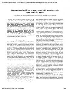
Pattern recognition is to assign a class to a given input value or a set of values [7,8]. Generally speaking, pattern recognition algorithms aim to provide a reasonable answer for all possible inputs and to perform most likely matching of the inputs, taking into account their statistical variation. This is contrasted with pattern-matching algorithms, which look for exact output that matches to the input in a pre-existing pattern or patterns. A common example of a pattern-matching algorithm is regular expression matching [9–11]. In contrast to pattern recognition, pattern matching is generally not considered as a type of machine learning but a type of artificial intelligence, although pattern-matching algorithms can sometimes succeed in providing similar-quality output to the sort provided by pattern-recognition algorithms. So far, there are some pattern-matching algorithms in the world, including ones for intervals. However, most of the interval-matching algorithms are used in much applied areas [12] and are highly related to specific features. In other words, these interval pattern matching methods are designed for specific problems, not for general ones. The main contribution of the paper is to propose an interval pattern matcher that makes use of the neural network, and we call it a “neural network-based interval pattern matcher”. This pattern matcher has the property that can identify a mathematical interval, instead of a real number. Experiments illustrate that neural networks can form the core of the “Neural Network-based Interval Pattern matcher” that can identify the patterns more quickly compared with the pattern-matching algorithm using a searching method once the training process finishes. The organization of this paper is as follows. In Section 2, we briefly introduce the preliminaries of the paper: neural networks. Section 3 describes the modeling of a neural network-based interval pattern matcher. Section 4 is the experiment to test the classifier that we propose. Finally, conclusions are given. 2. Preliminaries: Neural Networks Artificial neural networks (shown in Figure 1) are electronic neuron structures that simulate the neural structure of the brain. They process one training sample at one time and learn by comparing real output with targets. The errors from the initial training step are used to modify the network weights the second time around, and so on. Roughly speaking, an artificial neural network is composed of a set of input values (xi), associated weights (wij), and a function that sums the weights up and maps the results to the output vector (y). Neurons are organized into layers. The input layer is composed of neurons that represent the feature variable vector (x). The next layer is called the hidden layer; and there may be more than one hidden layer and more than one neuron in each hidden layer. The final layer is the output layer, where one node matches with one class for classification problems.
Figure 1. Artificial neural networks.
Information 2015, 6
390
Neural network is an important tool for classification [13,14]. Basically, a classifier takes objects as inputs and assigns each one to a class; objects are represented as vectors of features and classes are represented as class labels, such as 0 or 1. In the training phase, the correct class for each record is known, and the output nodes can therefore be assigned “class number” values—“1” for the node corresponding to the correct class, and “0” for the wrong class [15,16]. It is thus possible to compare the network's calculated output values with these “correct” (target) values, and calculate an error term for each node, which is the “Delta” rule. These errors are then used to adjust the weights in the hidden layers so that the output values will be closer to the “correct” (target) values for the next time. After the process of training, a single sweep forward through the network assigns a value to each output neuron, whose value is assigned to whichever class’s node had the highest value. It is well-known that there are several types of neural networks, each of which has unique functions. In our paper, we focus on the pattern matching ability using a neural network, and come up with a pattern matcher that is a neural network with additional data preparation layer. The traditional neural network is typical enough to be used to in our system illustrate our problem. 3. Neural Network-Based Interval Classifier Rules [17–19] are often stated as linguistic IF-THEN constructions. It has the general form “IF A THEN B”, where A is called the premise of the rule and B is the consequence. We use (A; B) to denote this rule. Neural network can express such rule efficiently. However, it is more often seen that both A and B take a more complex form. Take the simple rule set below as an example (R1) IF x1 is Small AND x2 is Small, THEN y is Small; (R2) IF x1 is Small’ AND x2 is Small’, THEN y is Small’. There are two rules in this example, and the number of inputs is two. Small and Small’ denote intervals over the universe of x and y. R1 can be denoted as (Small, Small; Small); R2 can be denoted as (Small’, Small’; Small’). Often, a continuous interval can be represented by some discrete examples. The discrete examples in the domain can be determined by interpolation. This idea reduces the processing complexity in our system using interval. For example, given the rule R1, we need some specific value or (values) to depict the interval Small to minimize the complexity of it, neural network would face the difficulty that one input values would face more than one output value. Details are shown as the following: If there is a one-to-many relationship between the inputs and targets in the training data, then it is not possible for any mapping to perform perfectly. One method is to calculate the average value for each interval. Any given network may or may not be able to approximate this mapping well at the beginning. However, it will form its best possible approximation to this mean output value when trained as well as possible. One problem emerges when average features cannot distinguish one interval from the others. Sometimes, different intervals may have the same average values, especially for the intervals having overlap values. Whatever method we use, one interval should be distinguishable from the others on the
Information 2015, 6
391
limited domain related to the problem that we are trying to solve. For example, if our domain is {Large, Small, Middle}, we need to distinguish these three intervals but do not need to distinguish others. Here, we have to emphasize the concept of “relation”. A “relation” is just a relationship among objects. If there are some persons in class and each person has their own height, the pair of one person and his/her name is a “relation”. Besides, these pairs are “ordered”, which means one comes first and the other comes second. The set of all the starting points is called “the domain” and the set of all the ending points is called “the range”. What should we notice is that all functions are relations but not all relations are functions. A function is a sub-classification of relation and a well-behaved relation, we mean that, given a starting point, we know exactly where to go; given an x, we get only and exactly one y. The relation {(7,8;0), (7,8;1)} where “7” and “8” are input values and “0” and “1” are output values, is not a function since certain xelements are paired with more than one unique y-element. However, the relation {(1;2), (3;2)} where “1” and “3” are input values and “2” is an output value, is a function since certain y-elements value can be paired with more than one unique x-element. It is well known that a neural network can approximate a function very well [20–22], but it cannot express the one-many mapping correctly since the weight changes would be compromised between different outputs given the same inputs. In a traditional neural network, the training error of a function would approximate zero when trained as well as possible [23–25]; while for the non-function relation, the error does not converge to a real number, but rather to an interval. For example, if we are given a relation {(1;2), (1;3)} and train the neural network using the training sample (1;2) and (1;3) alternately, at the beginning the weight change would simulate the relation (1;2) and then it would simulate the relation (1;3) and so forth. Thus, the weight changes would be a compromise among different outputs (“1” and “3”) given the same inputs (“1”) after a lot of iterations. When we input “1” to this well trained neural network, it would output a number between two and three randomly based on our research. Totally speaking, the range of the interval is closely related to the error interval. Here, we make use of this error interval to decide if the training process is finished or not in the training process. Besides, we can also use this error interval and testing outputs to identify different interval output in the testing process. Specifically, the error interval would fall within an interval that is closely related to the error interval and output some values that fall within the interval itself. The network structure of this example is shown in Figure 2.
Figure 2. Neural network-based interval matcher.
Information 2015, 6
392
Specification: Data preparation layer: This layer generates training samples from the raining rules. A suitable training sample is one which has values drawn from a distribution corresponding to a rule in the training rule base. (Training samples for rule R1 must obey R1.) The main goal of the input layer is to generate some training samples randomly, each of which contains independent variable values (x1, …, xn) and values of the induced variable (y) that obey the corresponding rule. We generate values for each of the variables by drawing from a rule distribution [26–28]. Using the example from Section 3, there are two independent variable values (x1, x2) and one induced value y. To generate a training example for rule R1, we would draw a sample for x1 from the Small region of the domain of X1; x2 would be drawn from the Small region for X2, and y would be drawn from the Small region of Y. For example, we would like to approximate the relation (A,B;C), where A is {1,2}, B is {3,4} and C is {6,7}. We decompose this relation into (1,3;6), (1,3;7), (1,4;6), (1,4;7), (2,3;6), (2,3;7), (2,4;6), (2,4;7). Input layer: This layer is similar to standard neural networks with inputs from the data preparation layer. Hidden layer: The function of this layer is similar to standard neural networks, except that we have separate networks for each set of input classes. The training itself is done using the Back-Propagation algorithm. During training, a training sample is only used to train a single network in the neural training layer, not all of them. Output layer: This layer outputs an interval values. if we input (1,3), (1,4), (2,3), (2,4), the output would be a number between 6 and 7 as would the others. Thus, we could estimate the interval C based on the outputs of the corresponding well trained neural network. 4. Experiments 4.1. Simple Test 4.1.1. Comparison Between Two Rules Using Our Program The reason why we conduct this experiment is to testify that the range of the interval is closely related to the error interval. We tested the range solution on the simple rules R1 and R2: Small is a set with the interval of [0, 10]. In other words, it is part of the “Small”. Table 1 depicts the experimental environment that we used for the tests. Table 1. Experimental environment. Algorithm to train the neural network
Back Propagation (BP) Algorithm
Neural network structure
4 layers having 3, 3, 3, and 1 neurons
Experiment tool
Matlab
We first test out the range solution on R1. For this example, the universal of all three variables is the interval [0, 100]. To generate a test example, we simply generate a random three-tuple in [0, 100]3, and then check if this conforms to the stated rule R1. (If it does not, we discard the training example.)
Information 2015, 6
393
In this experiment, we generate 42,803 training samples that satisfied the R1 in the rule set. Using 30,000 training samples to train the neural network, we get the error values shown below in Figure 3. Once the network finishes the training process, the error falls approximately within the interval [0–0.2]. 1.4
1.2
training error
1
0.8
0.6
0.4
0.2
0
0
0.5
1
1.5 training times
2
2.5
3 4
x 10
Figure 3. Training error using range solution of R1. Using the other 12,803 testing samples on the network, we get error values shown in Figure 4. We observe that the result approximately is between “0” to “0.2”. This means that the training process is successful and there is no over-fitting problem. 1.6 1.4 1.2
training error
1 0.8 0.6 0.4 0.2 0
0
0.5
1
1.5 training times
2
2.5
3 4
x 10
Figure 4. Training error using range solution of R2. We used another rule R2 to test the range solution. Using 20,000 training samples to train, the training error falls approximately within an interval [0, 0.08], as shown in Figure 5. Using the other 10,000 testing samples to test, the testing error falls approximately within an interval [0, 0.07], as shown in Figure 6.
Information 2015, 6
394 Error Histogram with 20 Bins
4
x 10
Training Zero Error
2
Instances
1.5
1
0.4742
0.4213
0.3684
0.3155
0.2626
0.2097
0.1568
0.1039
0.05095
-0.00196
-0.1078
-0.05487
-0.1607
-0.2136
-0.2665
-0.3194
-0.3723
-0.4252
-0.4781
0
-0.531
0.5
Errors = Targets - Outputs
Figure 5. Training error using “traingdx” of R1. Error Histogram with 20 Bins
4
x 10
Training Zero Error
2 1.8
Instances
1.6 1.4 1.2 1 0.8 0.6 0.4
0.194
0.1704
0.1468
0.1232
0.09967
0.07609
0.05251
0.02894
0.005361
-0.01822
-0.04179
-0.06537
-0.08894
-0.1125
-0.1361
-0.1597
-0.1832
-0.2068
-0.254
0
-0.2304
0.2
Errors = Targets - Outputs
Figure 6. Training error using “traingdx” of R2. It is observed that both rules’ training errors fall within an interval after getting a stable state, and the difference between the training errors of the two rules is the range of the error. The reason for this phenomenon is that the inputs of a training sample correspond to different output values. If the gap among the biggest output value and smallest output value is big, the range of the error is big; otherwise, the range of error is small. Although the training error also falls within an interval for a function, the range of the interval will approach zero as long as the training times are sufficient. This is different from the non-function relation, whose training error range would not approach zero no matter how many training times the training process would take [28–30].
Information 2015, 6
395
4.1.2. Comparison Between Two Rules Using Matlab Toolbox Table 2 depicts the experimental environment that we used for the tests. We use “traingdx” to replace the general BP algorithm to test our results; use standard Matlab toolbox (version R2014a) to generate our results, instead of our own programming. Table 2. Experimental environment. Algorithm to train the neural network
Gradient descent with momentum and adaptive learning rate backpropagation algorithm (traingdx)
Neural network structure
4 layers having 3, 3, 3, and 1 neurons
Experiment tool
Matlab neural network tool box
From Figures 5 and 6, we see the results are in accord with the last experimental results. Specifically, if we rotate the Figures 5 and 6 in clockwise direction about 90 degrees, these figures are almost the same as Figure 3 and Figure 4, respectively. With the increment of training times, the error would not decrease, but arrive to an interval, with the value vibrating within. The only difference is that Figures 5 and 6 have negative errors but Figures 3 and 4 do not. The reason for that is that we use absolute error to denote training errors. 4.2. Practical Test From Shanxi Provincial Meteorological Bureau, China, we got the ground surface meteorological observation data in Taiyuan, a city of Shanxi Province, China from May 2007 to October 2007, May 2008 to October 2008 and May 2009 to October 2009, which are the rainy seasons in that city. The specific meteorological elements included the day’s atmospheric pressure, relative humidity, dry and wet bulb temperature, wind speed and accumulated precipitation at 8 p.m. (Beijing Time, equivalent to 1200 UTC), which we took into our experiments. Table 3. Classification of input conditions. Atmospheric pressure
Dry and wet bulb temperature
Relative humidity
Wind speed
Rating
Value (hPa)
Rating
Value (°C)
Rating
Value (%)
Rating
Value (MPH)
Moderate
>940
Lowest