International Journal of Neural Systems, Vol. 8, Nos. 5 & 6 (October/December, 1997) 581–599 c World Scientific Publishing Company
A NEURAL NETWORK METHOD FOR IDENTIFICATION OF PROKARYOTIC AND EUKARYOTIC SIGNAL PEPTIDES AND PREDICTION OF THEIR CLEAVAGE SITES HENRIK NIELSEN, JACOB ENGELBRECHT∗ and SØREN BRUNAK Center for Biological Sequence Analysis, Department of Biotechnology, The Technical University of Denmark, DK-2800 Lyngby, Denmark GUNNAR VON HEIJNE Department of Biochemistry, Arrhenius Laboratory, Stockholm University, S-106 91 Stockholm, Sweden Received August 14, 1996 Accepted January 4, 1997 We have developed a new method for the identification of signal peptides and their cleavage sites based on neural networks trained on separate sets of prokaryotic and eukaryotic sequences. The method performs significantly better than previous prediction schemes, and can easily be applied to genome-wide data sets. Discrimination between cleaved signal peptides and uncleaved N-terminal signal-anchor sequences is also possible, though with lower precision. Predictions can be made on a publicly available WWW server: http://www.cbs.dtu.dk/services/SignalP/.
1. Introduction
The mechanism for targeting a protein to the secretory pathway is believed to be similar in all organisms and for many different kinds of proteins. 14 Signal peptides from widely different organisms are to some degree interchangeable.6 Therefore, it is quite surprising that signal peptides from different proteins do not share a strict consensus sequence — in fact, the sequence similarity between them is rather low. However, they do share a common structure. The most characteristic common feature of signal peptides is a stretch of seven to fifteen hydrophobic amino acids called the hydrophobic core or h-region. The region between the N-terminal of the preprotein and the h-region is termed the n-region. It is typically one to five amino acids in length, and normally carries positive charge. Between the h-region and the cleavage site is the c-region, which consists of three to seven polar, but mostly uncharged, amino acids.
Signal peptides control the entry of virtually all proteins to the secretory pathway, both in eukaryotes and prokaryotes.11,23,36 They comprise the N–terminal part of the amino acid chain, and are cleaved off while the protein is translocated through the membrane. Strong interest in automated identification of signal peptides and prediction of their cleavage sites has been evoked not only by the huge amount of unprocessed data available, but also by the industrial need to find more effective vehicles for production of proteins in recombinant systems. In this paper we address the organism-specific aspects of the problem and present neural-network based prediction methods to identify signal peptides and their cleavage sites in protein sequences from Gram-positive and Gramnegative bacteria, humans and other eukaryotes.
∗ Present
address: Novo Nordisk A/S, Scientific Computing, Building 9M1, Novo Alle, DK-2880 Bagsværd, Denmark.
581
582 H. Nielsen et al.
Close to the cleavage site a more specific pattern of amino acids is found. The (−3, −1)-rule states that the residues at positions −3 and −1 (relative to the cleavage site) must be small and neutral (at −1 almost always Ala, Gly, Ser, Cys or Thr) for cleavage to occur correctly.30,31 In contrast, position −2 is often occupied by an aromatic, charged or large polar residue. In bacterial signal peptides, the positive charge in the n-region is often balanced by a negative net charge in the c-region or in the first few residues of the mature protein.32 The most widely used method for predicting the location of the cleavage site has until recently been a weight matrix published in 1986.33 This method is also useful for discriminating between signal peptides and non-signal peptides by using the maximum cleavage site score. The original matrices are commonly used today, even though the amount of signal peptide data available has increased since 1986 by a factor of 5–10. Artificial neural networks, most often of the feedforward back-propagation type, have been used for many biological sequence analysis problems (for reviews see Refs. 12, 21). They have also been applied to the twin problems of predicting signal peptides and their cleavage sites, but until now without significant improvements in performance compared with the weight matrix method. Ladunga et al. 16 used an algorithm that adjusts the network architecture to the data for discriminating between signal peptides and non-signal peptides, but their network failed to outperform the discrimination ability of the weight matrix method, even though a larger database was used. Schneider and Wrede27 used neural networks trained by a genetic algorithm for predicting cleavage sites, but the data set was small and the performance did not even match that of the weight matrix method. An unsupervised neural network, the selforganizing feature map, was unexpectedly found to show a tendency for extracting sequences coding for the signal peptide region from a data set of human insulin receptor genes — A theoretically interesting but not easily applicable result.3 Here, we present a combined feed-forward neural network approach to the recognition of signal peptides and their cleavage sites, using one network to recognize the cleavage site and another network to
distinguish between signal peptides and non-signal peptides.19 A similar combination of two pairs of networks has been used with success to predict intron splice sites in pre-mRNA from humans and the dicotelydoneous plant Arabidopsis thaliana.8,15 2. Materials and Methods 2.1.
Extraction of signal peptide sequences
The signal peptide data were taken from SWISSPROT version 29.5 From a total of 38 303 entries, 5995 entries contained the keyword SIGNAL in the feature table. Entries suggesting absence of experimental evidence for the cleavage site were discarded, i.e. where the signal peptide was incomplete, the cleavage site was unknown, question marks or comments such as “POTENTIAL”, “PROBABLE”, or “BY SIMILARITY” were present, or an alternative cleavage site was suggested. This selection procedure reduces the number of cleavage sites which are not experimentally determined, but it does not eliminate them, since many SWISS-PROT entries simply lack information about the quality of the evidence, as we have previously found.20 Furthermore, all virus and phage genes were discarded. From the eukaryotic data set, proteins encoded by organellar (non-nuclear) genes were discarded (by excluding entries containing an “OG” line). From the prokaryotic data set, signal peptides cleaved by signal peptidase II (Lsp, a specific lipoprotein signal peptidase) were discarded, since the cleavage sites of these proteins differ considerably from those cleaved by the standard prokaryotic signal peptidase (Lep)35 ; this was done by excluding entries with a cross-reference to the PROSITE entry named “PROKAR_LIPOPROTEIN”.4 From each entry, the sequence of the signal peptide and the first 30 amino acids of the mature protein were included in the data set.a It would not be reasonable to give the entire protein sequence as background to the cleavage site, since the cleavage takes place while the protein is being translocated and the cleavage enzyme therefore hardly has the entire protein as a potential substrate. The value 30 is not arbitrary: several experimental results indicate that in E. coli the first 30 residues of the mature protein seem to have a function for protein export.2,24
a One entry, AVR9 CLAFU, which had less than 30 amino acids after the cleavage site was deleted.
Prediction of Signal Peptides 583
2.2.
Extraction of cytoplasmic and nuclear protein sequences
As background to the signal peptides, we extracted data sets comprising the N-terminal parts of cytoplasmic and (for the eukaryotes) nuclear proteins. This was done by searching for comment lines in SWISS-PROT specifying the subcellular location as “CYTOPLASMIC” or “NUCLEAR” without comments like “POTENTIAL” or “PROBABLE”. Entries comprising protein fragments were discarded (by searching for the word “FRAGMENT” in the description line or the keywords “NON_TER” or “NON_CONS” in the feature table), as were proteins shorter than 70 residues or lacking the initial Met. Virus and phage proteins were not included. The first 70 amino acids of each sequence were included in the data sets. In some cases (383 eukaryotic, 48 Gram-negative, and 14 Gram-positive) where the entry contained a feature table line with the key “INIT_MET”, indicating that the initiator methionine had been cleaved off, we prepended the missing “M” to the sequence. A few examples of disagreement between signal peptide and subcellular location information were found in the data: The entry MURF_ECOLI (E. coli UDP-MurNAc-pentapeptide synthetase) had both a signal peptide and a comment stating that it was located in the cytoplasm. The entry NO27_SOYBN (soybean nodulin-27) which was cytoplasmic according to the comment was very similar to two other nodulins (NO20_SOYBN and NO22_SOYBN) which both had signal peptides.b These four entries were deleted from the data set in the signal/non-signal peptide runs. According to our finished prediction method, MURF_ECOLI certainly does not look like a signal peptide, while the three nodulins look like typical signal peptides. 2.3.
Extraction of signal anchor sequences
Certain membrane proteins, known as type II membrane proteins, are attached to the membrane by an N-terminal sequence that shares many characteristics with a signal peptide but is not cleaved.34 Consequently, they consist of an N-terminal cytoplas-
mic domain, a single transmembrane domain, and a larger C-terminal extracellular or lumenal domain. In order to test whether the prediction method would erroneously classify these uncleaved signal peptides, also known as signal anchors, as signal peptides, a data set of signal anchors was extracted in the following way: In SWISS-PROT version 29, 157 entries contained the feature table keyword “TRANSMEM” with the qualifier “SIGNAL-ANCHOR (TYPE-II MEMBRANE PROTEIN)”. From these, we selected 137 eukaryotic signal anchors with specified endpoints and without comments like “POTENTIAL” or “PROBABLE”. Prokaryotic signal anchors were ignored, since only five of these were found (four of them potential). 18 entries were discarded because they contained more than one “TRANSMEM” line and therefore should be regarded as type IV (i.e. multi-spanning) membrane proteins, rather than type II. With one exception only, these proteins are members of the TM4 superfamily or bear similarity to it. Furthermore, we discarded 22 entries where the suggested signal anchor region (from the N-terminal of the protein to the C-terminal end of the specified transmembrane region) was 70 residues or longer, because these would hardly be mistaken for cleavable signal peptides. In many cases, the cytoplasmic domain preceding the signal anchor were marked “POTENTIAL” or “PROBABLE”, even if the signal anchor itself was not. We did not discard these entries, however; since the signal anchor data were not going to be used as training data but only as test data, we set the demands for the quality of experimental evidence lower than for the other data sets. From the 97 selected entries (28 of them human), the sequence of the N-terminal part of the protein up to 30 amino acids after the C-terminal end of the specified transmembrane region (signal anchor) was included in the data set, in analogy with the signal peptide data set. In nine cases (three of them human) where the entry contained a feature table line with the key “INIT_MET”, indicating that the initiator methionine had been cleaved off, we prepended the missing “M” to the sequence.
b A comment in NO27 SOYBN said that “Despite the similarity of their structures, the nodulins are located in different subcellular compartments.”
584 H. Nielsen et al.
2.4.
Division of data sets by systematic group
By using the information in the SWISS-PROT “OS” line, the resulting data sets were divided into prokaryotic and eukaryotic entries, and the prokaryotic data sets were further divided into Gram-positive eubacteria (Firmicutes) and Gramnegative eubacteria (Gracilicutes), excluding Mycoplasma and Archaebacteria. Additionally, two single-species data sets were selected, a human subset of the eukaryotic data, and an E. coli subset of the Gram-negative data. The numbers of signal peptides and cytoplasmic and nuclear proteins in the five organism groups are shown in Table 1. 2.5.
Redundancy reduction
Redundancy in the data sets was avoided by excluding pairs of sequences which had more than a certain number of identities (exact matches) in an alignment made with a protein identity matrix of high relative entropy.1 The cutoff value which gave the best separation between functionally homologous and nonhomologous signal peptide sequences was established for eukaryotes and prokaryotes separately: 17 identities for eukaryotes and 21 for prokaryotes. In this context, a sequence pair is defined to be functionally homologous if both cleavage sites are aligned at the same position.20 While investigating the pairwise similarities between signal peptide sequences, we found a number
of sequence pairs with similarity above the threshold but without aligned cleavage sites.20 By manually checking the references to these examples in the human signal peptide data set, a number of database errors were found. Five entries were found to lack experimental evidence for their cleavage sites: “ELNE_HUMAN”, “FCG3_HUMAN”, “FCGA_HUMAN”, “FCGB_HUMAN”, and “FCGC_HUMAN”. These have been discarded. Three entries were found to have the cleavage site indicated at a wrong position: “HA22_HUMAN”, “SOMV_HUMAN”, and “SOMW_HUMAN”. The cleavage sites of these have been changed accordingly. The other data sets have not been through this type of error checking. Therefore, the human signal peptide data set is probably more error-free than the other signal peptide data sets. We applied the same cutoff to non-signal-peptide sequences, even though the cutoff has been determined for signal peptide sequences specifically, since these merely serve as background to the signal peptide sequences. Redundancy reduction was not applied to the signal anchor data, since these were not going to be used as training data. After computing all pairwise alignments within each of the data sets, redundant sequences were removed using algorithm 2 of Hobohm et al.,13 which guarantees that no pairs of homologous sequences remain in the data set. This procedure removed 13–56% of the sequences. The numbers of nonhomologous signal peptide sequences remaining in the data sets are also shown in Table 1.
Table 1. The number of sequences in the data sets before (“tot.”) and after (“red.”) redundancy reduction. The organism groups are: Eukaryotes (“euk”), human, Gram-negative bacteria (“gram−”), E. coli (“ecoli”), and Gram-positive bacteria (“gram+”). The human data are subsets of the eukaryotic data, and the E. coli data are subsets of the Gram-negative data. No prokaryotic signal anchor sequences were used. The signal anchor sequences have not been redundancy-reduced.
euk
Signal Peptides tot. red.
Cytoplasmic Proteins tot. red.
Nuclear Proteins tot. red.
Signal Anchors tot.
2275
1011
854
269
1007
551
97
human
614
416
138
97
188
154
28
gram−
383
266
293
186
ecoli
119
105
128
119
gram+
187
141
123
64
− − −
− − −
− − −
Prediction of Signal Peptides 585
It is not surprising that the E. coli set was the least redundant, since protein families are known to be rare in E. coli.25 The largest degree of redundancy was found in the eukaryotic set which included protein families from single organisms as well as homologous proteins sequenced in many different organisms. Haemophilus influenzae sequences The Haemophilus influenzae Rd genome is the first genome of a free living organism to be completed.10 We have downloaded the sequences of all the predicted coding regions in the H. influenzae genome from the WWW server of The Institute for Genomic Research at http://www.tigr.org/. 2.6.
Neural network algorithms
The signal peptide discrimination problem was posed to the network in two ways: Recognition of the cleavage sites against the background of all other sequence positions, and classification of amino acids as belonging to the signal peptide or not. In the latter case, negative examples included both the first 70 positions of non-signal peptide proteins, and the first 30 positions after the cleavage site of proteins with signal peptides. Both symmetric and asymmetric versions of the windows were used, i.e. the number of positions included to the left and right of the site to be classified were varied independently. The amino acid sequence input was sparsely encoded when presented to the neural algorithms, using 21 input values for each position in the input window, one for each amino acid and one for “empty”, such that windows including positions to the left of the N-terminal could be encoded also. For each position in the window, the amino acid was coded by setting one of the 21 input units to 1.0 and all others to 0.0.8,22 The sequence data were presented to the network using moving windows of a size varying from 5 to 39 positions. Networks with 0 to 10 hidden units were used. Thus, the largest network used had 39 × 21 = 819 input values, and (819+1)×10+(10+1) = 8211 parameters (weights and thresholds). During training, the sequences were padded with a number of “empty” characters corresponding to the left-hand window size before the initial methionine, in order to represent the fact that some of the win-
dows are located close to the N-terminal of the protein. This may constitute important information for the signal peptide recognition system. However, we found that this padding did not change test performances significantly. The test performances reported in the results section are calculated without padding. Instead, at positions in the window which are outside the limits of the sequence, all input values are set to zero. The neural networks were trained using backpropagation. When training the networks we used the error function suggested by McClelland X log(1 − (Oiα − Tiα )2 ) , (1) E=− α,i
instead of the conventional error function26 X E= (Oiα − Tiα )2
(2)
α,i
where Oiα and Tiα are the output and target values respectively for training example α. This logarithmic error function reduced the convergence time considerably, and also had the property of making a given network learn more complex tasks (compared to the standard error measure) without increasing the network size. The learning rate was kept constant at 0.025. The weights were updated in on-line mode, with the training examples shuffled in random order for each training cycle. Training targets values were 1.0 for positive examples (cleavage sites or signal peptide positions) and 0.0 for negative examples. When evaluating the network output, a cutoff of 0.5 for positive assignment was always used. Based on the numbers of correctly and incorrectly predicted positive and negative examples, we calculate the correlation coefficient,17 defined as: (P t N t ) − (N f P f ) C=p , (N t + N f )(N t + P f )(P t + N f )(P t + P f ) (3) where P t and P f are the numbers of true and false positives, while N t and N f are the numbers of true and false negatives. The correlation coefficient of both training and test sets were monitored during training, and the performance of the training cycle with the maximal test set correlation was recorded for each training run. The networks chosen for further analysis and inclusion in the mail server have been trained until this cycle only.
586 H. Nielsen et al.
Test performances have been calculated by crossvalidation: Each data set was divided into five approximately equal-sized parts, and then every network run was carried out with one part as test data and the other four parts as training data. The performance measures were then calculated as an average over the five different data set divisions. 2.7.
Quantification of sequence information content
When a large set of sequences is aligned the Shannon entropy of information measure29 can be used to quantify the randomness in each column. The information content, defined as the difference between maximal and actual entropy, is computed by the formula X nj (α) nj (α) Ij = Hmax − Hj = log2 20 + log2 , N Nj j α (4) where nj (α) is the number of occurrences of the amino acid α and Nj is the total number of letters (occupied positions) at position j. The unit of information is bits. The information content is displayed in the form of sequence logos,28 where the amino acid symbols are used to represent the value of I at a given position. The sum of the height of the letters indicates the value of I, and the height of each letter represents its frequency at that position. 3. Results 3.1.
Characterisation of the signal peptides
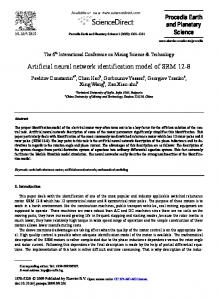
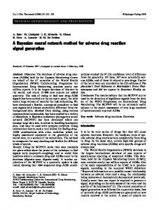
The length distribution of the signal peptides is shown in Fig. 1. Signal peptides from Gram-positive bacteria are considerably longer than those of other organisms. This has previously been observed in a similar but less comprehensive study.38 Signal peptides shorter than 15 are extremely rare and may represent errors in the database. This may also be the case for the other extreme of the distribution, i.e. signal peptides longer than, say, 35 for eukaryotes, 40 for Gram-negative bacteria, and 45 for Grampositive bacteria. The sequence patterns at the cleavage site are shown as sequence logos28 in Fig. 2. The sequence logo depicts an alignment of signal peptide sequences
Fig. 1. Distribution of lengths of the eukaryotic and prokaryotic signal peptides. The average length is 22.6 amino acids for eukaryotes, 25.1 for Gram-negative bacteria, and 32.0 for Gram-positive bacteria.
aligned by the cleavage sites. The cleavage site pattern shows differences between eukaryotes and prokaryotes. The (−3, −1) rule is clearly visible for all three data sets; but while a number of different amino acids are accepted in the eukaryotes, the prokaryotes accept almost exclusively Alanine in these two positions. In the first few positions of the mature protein (downstream of the cleavage site) the prokaryotes show certain preferences for Ala, negatively charged (D or E) amino acids, and hydroxy amino acids (S or T), while no pattern can be seen for the eukaryotes. The h-region is clearly visible, in the prokaryotes dominated by Leu (L) and Ala (A) in approximately equal proportions, and in the eukaryotes dominated by Leu with some occurrence of Val (V), Ala, Phe (F) and Ile (I). Note that the h-regions of Grampositive bacteria are much more extended than those of Gram-negative bacteria or eukaryotes. In the leftmost part of the alignment, the positively charged residue Lys (K) (and to a smaller extent Arg (R)) is seen in the prokaryotes; while the eukaryotes show a somewhat weaker occurrence of Arg (barely visible in the figure) and almost no Lys. This corresponds well with the hypothesis that positive residues are required in the n-region for prokaryotes where the N-terminal Met is formylated, but not necessarily for eukaryotes where the N-terminal Met in itself carries a positive charge.31 Met (M), indicating the N-terminals of the sequences, can be seen in both logos.
Prediction of Signal Peptides 587
Fig. 2. Sequence logos of signal peptides, aligned by their cleavage sites. The total height of the stack of letters at each position shows the amount of information, while the relative height of each letter shows the relative abundance of the corresponding amino acid. Positively and negatively charged amino acids are shown in blue and red respectively, while uncharged amino acids are coloured from light green to dark green according to their hydrophobicity according to the GES scale.9
As far as length distribution and sequence logos are concerned, human signal peptides show no significant differences compared to those of all eukaryotes, nor did signal peptides of E. coli compared to those of Gram-negative bacteria in general. 3.2.
Network architecture and single-position performance
The trained networks provide two different scores between zero and one for each position in an amino acid sequence. The output from the signal/
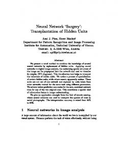
non-signal peptide networks, the S-score, can be interpreted as an estimate of the probability of the position belonging to the signal peptide, while the output from the cleavage site/non-cleavage site networks, the C-score, can be interpreted as an estimate of the probability of the position being the first in the mature protein (position +1 relative to the cleavage site). In Fig. 3, two examples of the values of C- and Sscores for signal peptides are shown. A typical signal peptide with a typical cleavage site will yield curves
588 H. Nielsen et al.
(a)
(b) Fig. 3. Examples of predictions for sequences with verified cleavable signal peptides. The values of the C-score (output from √ cleavage site networks), S-score (output from signal peptide networks), and Y-score (combined cleavage site score, Yi = Ci ∆d Si ) are shown for each position in the sequences. The C- and S-scores are averages over five networks trained on different parts of the data. Note: The C-score is trained to be high for the position immediately after the cleavage site, i.e. the first position in the mature protein. The true cleavage sites are marked with arrows. (a) is an example of a sequence with all positions being correctly predicted according to both C-score and S-score. (b) has two positions with C-score higher than 0.5 — the true cleavage site would be incorrectly predicted when relying on the maximal value of the C-score alone, but the combined Y-score is able to predict it correctly.
as those shown in Fig. 3(a), where the C-score has one sharp peak that corresponds to an abrupt change in S-score. In other words, the example has 100% correctly predicted positions, both according to Cscore and S-score. Less typical examples may look like Fig. 3(b), where the C-score has several peaks. For each of the five data sets, one signal/nonsignal peptide network architecture and one cleavage site/non-cleavage site network architecture was chosen on the basis of test set correlation coefficients. We did not pick the architecture with the absolute best performance, but instead the smallest network that could not be significantly improved by enlarging the input window or adding more hidden units. The correlation coefficients were cross-validated (averaged over the five different data set partitions) before this analysis. The optimal network architecture and correlation coefficients for all the data sets are shown in Table 2.
As mentioned in the Methods section, the cutoff for assigning a positive was 0.5 for both C-score and S-score. This was also found to be the optimal cutoff value according to correlation coefficient, except for the Gram-positive data set where the C-score correlation coefficient could be increased to 0.56 by lowering the cutoff to 0.4. As is apparent in Table 2, the C-score problem is best solved by networks with asymmetric windows, i.e. windows including more positions upstream than downstream of the cleavage site. This corresponds well with the location of the cleavage site pattern information as shown in Fig. 2. It is also in good correspondence with the logos that the left-hand window size is much larger for the Gram-positive data set than for the others. However, it is surprising that the performance for the Gram-negative data set could not be enhanced by enlarging the left-hand window beyond position −11.
Prediction of Signal Peptides 589
Table 2. Optimal neural network architecture and prediction accuracy for classifying single positions. “C-score” refers to prediction of cleavage sites versus non-cleavage sites, while “S-score” refers to prediction of signal peptide positions versus non-signal peptide positions. CC and CS are the correlation coefficients for C-score and S-score, respectively. Correlation coefficients are cross-validated averages over five test sets. The cutoff for positive assignment (cleavage site for the C-score and signal peptide position for the S-score) is 0.5 in all cases. The columns labeled “window” and “h-units” show the configuration of the input window and the number of hidden units in the optimal network. The C-score windows include a number of positions to the left and right of the potential cleavage site, while the S-score windows include the position to be classified plus a number of positions to the left and the right. Results are shown for each data set (see Table 1 for abbreviations). “human by euk” refers to results obtained when using networks trained on all eukaryotic data to test human data; while “ecoli by gram−” refers to results obtained when using networks trained on all Gram-negative data to test E. coli data.
window
C-score h-units
window
S-score h-units
CC
human
15 + 4
2
0.61
13 + 1 + 13
4
0.89
euk
17 + 2
2
0.60
13 + 1 + 13
4
0.90
human by euk
−00 −
−00 −
0.58
−00 −
−00 −
0.90
ecoli
15 + 2
2
0.76
21 + 1 + 17
0
0.83
gram−
11 + 2
2
0.73
9+1+9
3
0.81
ecoli by gram−
−00 −
−00 −
0.80
−00 −
−00 −
0.83
gram+
21 + 2
0
0.54
9+1+9
3
0.82
The S-score problem, on the other hand, is apparently best solved by symmetric windows, the only exception being the network trained on the small E. coli set where the slightly skewed 21 + 1 + 17 did perform better than a symmetric window. However, the E. coli set was equally well predicted by the network trained on the Gram-negative data, using a much smaller window. The difference between the optimal architectures for different data sets may appear large but they do not necessarily reflect a significant variation between the characteristics of the data sets. It seems remarkable that the E. coli set shows an optimal SP window of 21 + 1 + 17 when the optimal SP window for the Gram-negative set is only 9 + 1 + 9; but this should be seen in comparison with the hidden layer size. The difference between the 21 + 1 + 17 network without hidden units and the 9 + 1 + 9 network with 3 hidden units is not very large, neither with respect to performance nor to total number of free parameters in the neural network. 3.3.
CC
Predicting cleavage site location using the C-score
The networks described in the previous section are selected for the best correlation coefficient when a
cutoff of 0.5 for the assignment of single positions is used. However, the performance of the C-score networks may also be measured at the sequence level by assigning the cleavage site of each signal peptide to the position in the sequence with the maximal C-score and calculating the percentage of sequences with the cleavage site correctly predicted by this assignment. This is how the performance of the weight matrix method33 is calculated. Evaluating the network output at the sequence level can improve the performance; even when the C-score has no peaks or several peaks above the cutoff value, the true cleavage site is often found at the position where the C-score is highest. The training process has been investigated in closer detail for the C-score networks in order to check the correspondence between single-position and sequence level performance. This has been done for the architectures found in the previous section only, since the sequence level evaluation requires too much computation to carry out for every possible architecture. In an earlier study using smaller data sets18 we found that the optimal architectures did not differ significantly from single-position to sequence level performance. When analyzing the training process, however, we found that the sequence level performance in
590 H. Nielsen et al.
Table 3. Neural network prediction accuracy for locating cleavage sites in signal peptide sequences using cleavage site (C-score) networks. The columns labeled “% correct” show the percentage of sequences with correctly predicted cleavage sites (cross-validated averages over five test sets), where the cleavage site is predicted to be at the position where the C-score is highest. The network architectures are the same as in Table 2. In the left half of the table, the training of the networks was stopped at the cycle where single-position performance (CC ) was optimal, as is the case in Table 2. In the right half of the table, the training was stopped at the cycle where sequence-level performance (% correct) was optimal. The columns labeled “cycle” show the average number of cycles the networks were trained. C-score Optimized by:
single position (CC )
entire sequence (% correct)
cycle
% correct
cycle
% correct
human
26.4
63.2
20.8
66.8
euk
17.6
67.5
13.8
69.6
human by euk
−00 −
66.0
−00 −
67.4
ecoli
34.4
76.0
17.8
82.7
gram−
26.4
73.2
27.0
78.1
ecoli by gram−
−00 −
81.3
−00 −
86.8
gram+
21.8
60.7
8.4
66.4
almost every training run peaked at an earlier point in the training than the single-position performance did. In Table 3 the sequence level performance is shown for two versions of the networks, stopped at the point in the training where either the singleposition or the sequence level performance was optimal. For the final prediction method we have chosen those versions optimized for sequence level performance. For every cycle in the training process, we calculated the sequence level performance, the average scores for both categories, and the single-position correlation coefficient for a range of cutoffs at intervals of 0.01. Since the data set is very skewed (i.e. the number of cleavage site positions is much smaller than the number of non-cleavage site positions), the network initially reduces the error by forcing the output to be close to zero for all examples, and then it gradually raises the output value for the positive examples selectively. The optimal cutoff (i.e. the cutoff that gives the best correlation coefficient) tends to grow during the training process. When the network training is stopped before the single-position correlation coefficient (for a cutoff of 0.5) reaches maximum, the scores for the positive examples are therefore often lower than 0.5, and a smaller cutoff value may give a better separation between positive and negative examples.
The five networks trained on different data partitions are optimized individually for sequence level performance, i.e. they have been stopped at different points in the training. This has made it necessary to modify the C-score values in order to make the output from the five different networks comparable. We have scaled the output of each individual network so that the optimal cutoff for single-position performance is 0.5, also for the networks optimized for sequence level performance. 3.4.
Predicting cleavage site location using a combined score
If there are several C-score peaks of comparable strength, the true cleavage site may often be found by inspecting the S-score curve in order to see which of the C-score peaks that coincides best with the transition from the signal peptide to the non-signal peptide region. In order to formalize this and improve the prediction, we have tried a number of linear and non-linear combinations of the raw network scores and evaluated the percentage of sequences with correctly placed cleavage sites in the five test sets. The best of the mathematically simple measures was the geometric average of the C-score and a smoothed derivative of the S-score. We have termed this combined measure the Y-score:
Prediction of Signal Peptides 591
Table 4. Neural network prediction accuracy for locating cleavage sites in signal peptide sequences using a combined score (Y-score) of cleavage site and signal peptide networks. The Y-score is the geometric average of the Cscore and a derivative of the S-score √ calculated over a window of 2d positions: Yi = Ci ∆d Si . The optimal value for d is shown for each data set. As in Table 3, “% correct” is the percentage of sequences with correctly predicted cleavage sites. The network architectures are the same as in Table 2. For the “human by euk” and “ecoli by gram−” results, the d values are those determined for the “euk” and “gram−” networks respectively.
d
Y-score % correct
human
8
68.0
euk
17
70.2
−00 −
67.9
human by euk ecoli
7
83.7
gram−
19
79.3
−00 −
85.7
8
67.9
ecoli by gram− gram+
Yi =
p Ci ∆d Si ,
(5)
where ∆d Si is the difference between the average S-score of d positions before and d positions after position i: d d−1 X 1 X ∆d Si = Si−j − Si+j . (6) d j=1 j=0 For each data set, we chose the d value that resulted in the best sequence level performance. The d values and the resulting prediction accuracies are given in Table 4. The difference between the results of d values was not large for d ≥ 7. Consequently, the different optimal d values for different data sets probably does not reflect a significant variation between the data sets. The Y-score gives a certain improvement in sequence level performance (% correct) relative to the C-score, but the single-position performance (CC ) is not improved (results not shown). An example where the C-score alone gives a wrong prediction while the Y-score is correct is shown in Fig. 3(b). 3.5.
Predicting sequence type
In addition to locating the cleavage site, the neural network scores can be used to predict whether a
test sequence has a signal peptide (i.e. is the start of a secretory protein) or no signal peptide (i.e. is the start of a cytoplasmic or, in eukaryotes, nuclear, mitochondrial, or peroxisomal protein). In Fig. 4, two examples of C-, S-, and Y-scores in non-secretory proteins are shown, as a contrast to the scores for signal peptide sequences shown in Fig. 3. The simplest method of discrimination is to use the maximal values of the scores in each sequence. As the example in Fig. 4(b) shows, the C-score or S-score used in isolation may lead to false positives. The maximal values of the Y-score or the S-score are both significantly better discriminators than the C-score (results are shown in Table 6). The best measure, however, is the average of the S-score in the predicted signal peptide region, i.e. from position 1 to the position immediately before the position where the Y-score has maximal value. In particular for the Gram-positive bacteria, this proved to be significantly better than the maximal Y-score or maximal S-score. In addition, the distributions of the “mean S-score” measure for signal and nonsignal sequences are nicely symmetrical and very well separated, with modes close to 0.1 and 0.9. The distributions for the eukaryotic data are shown as an example in Fig. 5. If the Y-score reaches its maximal value at a very early position in the sequence of a non-signal peptide, the mean S-score may be misleading because it is averaged over a few positions only. In order to check whether this is a significant source of false positive predictions, we have investigated the distribution of Y-score maximum positions among the sequences predicted to be signal peptides, but did not find more unusually short predicted lengths among the false positives than among the true positives. 3.6.
Weight matrix results
In order to compare the strength of the neural network approach to a more traditional computational method, we have compared our results with the weight matrix method used by von Heijne in 1986.33 All performances in that study were sequence level performances, given as percent correctly placed cleavage sites. The reported training performance — i.e. the performance of matrices constructed from the whole sample and tested on the whole sample — was 87% for 161 eukaryotic sequences and 100% for
592 H. Nielsen et al.
(a)
(b) Fig. 4. Examples of predictions for sequences of non-secretory proteins (cf. Fig. 3). A typical example is shown in (a) (a cytoplasmic protein), where all three scores are very low throughout the sequence. In (b) (a nuclear protein), the maximal values of C-score and S-score are in fact above the cutoff values, but the C-score peak occurs far away from the S-score decline, and the region of high S-score is too short. Maximal Y-score and and mean S-score are well below their cutoffs, making a correct prediction possible also in this case.
Fig. 5. Distribution of the mean signal peptide score (S-score) for signal peptides and non-signal peptides (eukaryotic data only). “Non-secretory proteins” refer to the N-terminal parts of cytoplasmic or nuclear proteins, while “Signal anchors” are the N-terminal parts of type II membrane proteins. The mean S-score of a sequence is the average of the S-score over all positions in the predicted signal peptide region (i.e. from the N-terminal to the position immediately before the maximum of the Y-score). The bin size of the distribution is 0.02.
Prediction of Signal Peptides 593
36 prokaryotic sequences. Test performance — calculated by cross-validation, as in the present work — was 78% for eukaryotes (average of seven subsamples) and 89% for prokaryotes (average of four subsamples). We have followed the method of von Heijne33 with one minor exception: Instead of using standard average amino acid frequencies measured for soluble proteins in general, we calculate the average amino acid frequencies from the training set used for constructing the matrix. In an earlier work, we found this approach to give better results.18 While using the weight matrices, we regard zero counts at the positions −1 and −3 relative to the cleavage site as significant because of the (−3, −1)rule. At all other positions, counts of 0 are regarded as effects of limited data set size, so they are treated as counts of 1. We have only compared the performance for cleavage site location using the maximal value of the neural network C-score or the corresponding weight matrix score. We have not tried to assign a cutoff value for cleavage site assignment and therefore no single-position correlation coefficient is available. The performances given in Table 5 are calculated at the sequence level, as in Tables 3 and 4. Previously, we have found that the weight matrix is unable to solve the problem of distinguishing signal peptide positions from non-signal peptide positions.18 Therefore, no attempt was made here to calculate scores equivalent to the S- or Y-scores using weight matrices. In a pilot study made with a smaller data set, we found that the performance in calculating cleavage site score was smaller for the weight matrix than for the neural networks. Even neural networks without hidden units were found to perform slightly better than the weight matrices.18 With the full data sets, however, the weight matrix method was not always weaker than the C-score neural networks (compare Table 5 to Table 3). It performed equally well as or better than these neural networks for the Gram-negative, E. coli, and human data sets. With the Gram-positive data set, the neural networks became better than the weight matrix method after optimization for sequence level performance, and only with the eukaryotic data set did the neural networks outperform the weight matrix method without special optimization.
Table 5. Weight matrix prediction accuracy for locating cleavage sites in signal peptide sequences. “% correct” is the percentage of sequences with correctly predicted cleavage sites, where the cleavage site is predicted to be at the position where the weight matrix score is highest. Weight matrix window % correct human
15 + 8
66.7
euk
17 + 8
65.9
−00 −
63.7
ecoli
15 + 2
83.8
gram−
15 + 4
78.9
human by euk
ecoli by gram− gram+
−00 −
83.8
21 + 2
63.6
The combination of cleavage site and signal peptide networks (the Y-score, compare Table 5 to Table 4) improves the performance of the network method to a higher level than the weight matrix method for most of the data sets, though only to the same level for the Gram-negative and E. coli sets. The optimal matrix windows were in three cases (eukaryotic, human, and Gram-negative) larger than those found to be optimal for neural networks. This is not peculiar, since the networks in these cases had two hidden units and therefore more parameters. The results are considerably worse than the 78% and 89% found by von Heijne in 1986, even though the optimal windows are larger. This may reflect a larger variation in the examples of the signal peptides found since then. It may, of course, also reflect a higher occurrence of errors in our automatically selected data than in the manually selected 1986 set. The optimal window size for the weight matrix is equal to or larger than the optimal window size for the neural networks (compare Table 5 to Table 2). The difference in optimal window size is remarkable for the Gram-negative data set, where the neural networks performed worse than the weight matrices. In order to check whether the poor performance of the neural networks in this case was due to an inappropriate choice of window size, we analysed the training process in detail on Gram-negative data also for networks with the 15 + 4 window (using both 0 or 2 hidden units), but the sequence level performance did not improve relative to the 11 + 2 window.
594 H. Nielsen et al.
Table 6. Neural network prediction accuracy for classification of sequences as signal peptides or non-signal-peptides, measured by the correlation coefficient (CSP ). Four different classification measures are compared: The maximal values in the sequence of the raw cleavage site score (“C-score”), signal peptide score (“Sscore”), or combined cleavage site score (“Y-score”); and the mean value of the signal peptide score (“S-score”) averaged from position 1 to the best cleavage site (according to the Y-score). The cutoff for positive assignment (i.e. predicting that the sequence in question is a signal peptide) is in the range 0.37–0.57 for maximal C-score, 0.28–0.36 for maximal Y-score, 0.71–0.95 for maximal S-score, and 0.44–0.55 for mean S-score. The network architectures are the same as in Table 2. Correlation coefficients are cross-validated averages over five test sets.
3.7.
Maximal C-score CSP
Maximal Y-score CSP
Maximal S-score CSP
Mean S-score CSP
human
0.71
0.95
0.95
0.96
euk
0.85
0.97
0.96
0.97
human by euk
0.85
0.98
0.97
0.97
ecoli
0.67
0.88
0.89
0.89
gram−
0.71
0.89
0.82
0.88
ecoli by gram−
0.75
0.94
0.83
0.92
gram+
0.64
0.85
0.87
0.96
Signal peptides versus signal anchors
Signal anchors often have sites similar to signal peptide cleavage sites after their hydrophobic (transmembrane) region. Therefore, a prediction method can easily be expected to mistake signal anchors for peptides. In Fig. 5, the distribution of the mean S-score for the 97 eukaryotic signal anchors is included. It shows some overlap with the signal peptide distribution. If the cutoffs from Table 6 are applied to the signal anchor data sets, 50% of the eukaryotic signal anchor sequences are falsely predicted as signal peptides (the corresponding figure for the human signal anchors is 75% when using human networks and 68% when using eukaryotic networks). With a cutoff optimized for signal anchor versus signal peptide discrimination (0.62), we were able to lower this error rate to 45% for the eukaryotic data set. The mean S-score still gives a better separation than the maximal Cor Y-score, which indicates that the pseudo-cleavage sites are in fact rather strong. However, the pseudo-cleavage sites often occur further from the N-terminal than genuine cleavage sites do. If we do not accept signal peptides longer than 35 (this will exclude only 2.2% of the eukary-
otic signal peptides in our data set), the percentage of false positives among the signal anchors drop to 28% for the eukaryotic, and 32% for the human signal anchors (39% when using eukaryotic networks). 3.8.
Scanning the Haemophilus influenzae genome
We have applied the prediction method with networks trained on the Gram-negative data set to all the amino acid sequences of the predicted coding regions in the Haemophilus influenzae genome. Only the first 60 positions of each sequence were analyzed. The distribution of mean S-score (from position 1 to the position with maximal Y-score) is shown in Fig. 6. When applying the optimal cutoff value found for the Gram-negative data set (0.54) we obtained a crude estimate of the number of sequences with cleavable signal peptides in H. influenzae: 330 out of 1680 sequences, or approximately 20%. If maximal S-score is used instead of mean S-score, the estimate comes out as 28%, and with maximal Y-score it is 14% (distributions not shown). If all three criteria are applied together, leaving only “typical” signal peptides, we get 188 sequences (11%).
Prediction of Signal Peptides 595
Fig. 6. Distribution of the mean signal peptide score (S-score) for all predicted Haemophilus influenzae coding sequences. The mean S-score is calculated using networks trained on the Gram-negative data set. The bin size of the distribution is 0.02. The arrow shows the optimal cutoff for predicting a cleavable signal peptide. The predicted number of secretory proteins in H. influenzae (corresponding to the area under the curve to the right of the arrow) is 330 out of 1680 (20%).
Some of the sequences predicted to be signal peptides according to S-score but not according to Y-score may be signal anchor-like sequences of type II (single-spanning) or type IV (multi-spanning) membrane proteins. If we apply the slightly higher cutoff optimised for discrimination of signal anchors versus signal peptides in eukaryotes (0.62) to the mean S-score, the estimate is lowered from 20% to 15%. As a test of this hypothesis, we have made a hydrophobicity analysis of the entire sequences of the H. influenzae predicted coding regions as described in Ref. 37. We did not apply the positive-inside rule but only counted the number of regions with hydrophobicity larger than a specified cutoff in order to get a crude estimate of the number of transmembrane segments in each protein. Among the 188 “typical” signal peptides, there are 54 (29%) with more than one predicted transmembrane segment (including the h-region of the signal peptide itself); while as many as 69 (50%) of the 139 sequences which are predicted to be signal peptides according to the mean S-score but not the maximal Y-score have more than one predicted transmembrane segment. It has been observed that cleavable signal peptides are rarely found in bacterial cytoplasmic membrane proteins,7 and, as mentioned in the data section, very few bacterial proteins have a confirmed
N-terminal signal anchor. It is therefore possible that a better estimate of the proportion of secretory proteins might be achieved by combining the signal peptide prediction with a more sophisticated prediction of transmembrane segments and excluding those that have multiple transmembrane segments. We have not done this with the present hydrophobicity analysis method, since it is optimized to locate the transmembrane regions of membrane proteins rather than to discriminate between soluble and membrane proteins. On the other hand, the mean S-score may also give under-predictions, if the initiation codon of the predicted coding region has been placed too far upstream. In this case, the apparent signal peptide becomes too long, and the region between the false and the true initiation codon will probably not have signal peptide character, possibly bringing the mean S-score of the erroneously extended signal peptide region below the cutoff. In this analysis, there were 51 H. influenzae sequences predicted to be signal peptides according to the maximal Y-score but not the mean S-score; and these did indeed have an average predicted length of 35.5 amino acids as contrasted to the average length of 25.2 for the 188 typical signal peptides (which corresponds perfectly with the average length of 25.1 for the Gram-negative data set). An additional observation suggesting that these
596 H. Nielsen et al.
51 sequences might contain false initiation codons is that 41 (80%) of them contain a Methionine between position 2 and 60, while the corresponding number for the 188 typical signal peptides is only 63%. In conclusion, the scanning of the H. influenzae genome illustrates both the strengths and pitfalls of the current prediction method when it is applied on a whole-genome basis. 3.9.
Method and data publicly available
The finished prediction method is available both via an e-mail server and a World Wide Web server. Users may submit their own amino acid sequences in order to predict whether the sequence is a signal peptide, and if so, where it will be cleaved. We recommend that only the N-terminal part (say, 50–70 amino acids) of the sequences is submitted, so that the interpretation of the output is not obscured by false positives further downstream in the protein. The user is asked to choose between the network ensembles trained on data from Gram-positive, Gram-negative, or eukaryotic organisms. We did not include the networks trained on the single-species data sets in the servers, since these did not improve the performance. The values of C-score, S-score, and Y-score is returned for every position in the submitted sequence. In addition, the maximal Y-score, maximal S-score, and mean S-score values are given for the entire sequence and compared with the appropriate cutoffs. If the sequence is predicted to be a signal peptide, the position with the maximal Y-score is mentioned as the most likely cleavage site. A graphical plot in postscript format, similar to Figs. 3 and 4, may be requested from the servers. We strongly recommend that a graphical plot is always used for interpretation of the output. The address of the mail server is
[email protected]. For detailed instructions, send a mail containing the word “help” only. The World Wide Web server is accessible via the Center for Biological Sequence Analysis homepage at http://www.cbs.dtu.dk/. All the data sets mentioned in Table 1 are available from an FTP server at ftp://virus.cbs.dtu.dk/pub/signalp. Retrieve the file README for detailed descriptions of the data and the format. The FTP server and the mail server
can both be accessed directly from the World Wide Web server. 4. Discussion A new method which is able to identify secretory signal peptides and predict their cleavage sites with high accuracy, both in prokaryotes and eukaryotes, has been developed. The prediction performance reported in this study corresponds to minimal values. The test sets in the cross-validation have very low sequence similarity; in fact, the sequence similarity is so low that the correct cleavage sites cannot be found by alignment.20 This means that the prediction accuracy on sequences with some similarity to the sequences in the data sets will in general be higher. Signal peptides of eukaryotes, Gram-negative bacteria, and Gram-positive bacteria differ in their structure, as the sequence logos (Fig. 2) show. This difference is reflected in the performances in various ways. Gram-negative cleavage sites have the strongest pattern — i.e. the highest information content — and consequently they are the easiest to predict, both at the single-position and at the sequence level. The eukaryotic cleavage sites are significantly more difficult to predict, both according to C-score, Y-score, and weight matrix score. Gram-positive cleavage sites are slightly more difficult to predict than the eukaryotic, which would not be expected from the sequence logos (Fig. 2), since they show nearly as high information content as the Gramnegative cleavage sites. On the other hand, the Gram-positive signal peptides are by far the longest, as seen in Fig. 1, which means that the cleavage sites have to be located against a larger background of non-cleavage site positions. The S-score, which distinguishes positions in the signal peptides from non-signal peptide positions, shows the opposite pattern: the correlation for the S-score is higher for the eukaryotes than for the prokaryotes. This is may be due to the more characteristic leucine-rich h-regions of the eukaryotic signal peptides, which are also apparent in the sequence logos (Fig. 2). Using single-species data sets did not improve the performance. The human signal peptides are predicted equally good by the eukaryotic networks as by the human networks, and the E. coli signal peptides
Prediction of Signal Peptides 597
are predicted even better by the Gram-negative networks than by the E. coli networks. In other words, we have found no evidence of species-specific features of the signal peptides of humans and E. coli. The poorer performance of the E. coli networks relative to the Gram-negative networks can be explained by the relatively small size of the E. coli data set. In the cleavage site versus non-cleavage site problem, the window that gave the optimal cleavage site location was from 11 to 17 signal peptide residues, and 2 to 4 non-signal peptide residues, depending on the organism class. Larger windows gave a slightly lower performance. These windows are larger than those found to be optimal in an earlier weight-matrix based method33 : 13 + 2 for eukaryotes and 5 + 2 for prokaryotes.c Consequently, there must be some information located outside of von Heijne’s windows that is important for cleavage site recognition, but is only picked up by the neural networks when using the larger amount of data. The optimal windows for the networks trained to recognize cleavage sites (C-score) are highly asymmetric. This suggests that the pattern defining the cleavage site is located mainly in the signal peptide. This corresponds well with the amount of information in the sequences aligned by the cleavage site (Fig. 2). The optimal window size for the networks trained to distinguish residues in signal peptides from residues in the mature part of the proteins (S-score) was found to be 13 + 1 + 13 for eukaryotes and 9 + 1 + 9 for prokaryotes (except the E. coli set where 21 + 1 + 17 was found to be better), i.e. these windows are symmetric. In other words: to decide whether a given amino acid in a sequence belongs to the signal peptide, it is equally important to examine the preceding (upstream) positions as the following (downstream) ones. The windows of the C-score and S-score networks may be seen as examples of local windows, recognizing specific sites, and global windows, recognizing extended sequence domains, respectively. A combination of networks with local and global windows attacking a biological sequence recognition problem has previously been used with substantial success.8,15 Here, the local networks were trained to
locate splice sites (donor or acceptor sites) in human messenger RNA precursor (pre-mRNA), while the global network was trained to discriminate between coding and non-coding nucleotide sequences. The method of combination was similar to the weighted sum used in this project, except that all the evaluation took place at the single-position level instead of the sequence level. In the pre-mRNA study, the combined method was found to perform considerably better than either the local or global networks alone. Since the combination of C-score and S-score networks (Y-score) led to only a modest increase in performance, it would appear that the difference between the types of information recognized in the local and global approaches was smaller for the signal peptide networks than for the pre-mRNA splice site networks. However, the value of the global S-score should not be underestimated. It constitutes information different from the local C-score which may be useful in many contexts. Thus, individual sequences may be scanned with the networks, and the scores plotted together with the sequence as in Figs. 3 and 4. Plots like these may be analyzed manually, and in combination with knowledge of the protein in question the curves may give valuable clues to if and where one or more cleavage sites may be found. Furthermore, the mean S-score may be used to discriminate uncleaved signal peptides (signal-anchors) from cleaved signal peptides, as shown in Fig. 5. In many cases, the network scores may give information of phenomena which have not been discovered experimentally. For example, the plot in Fig. 3(b) where the C-score shows two distinct peaks may suggest that the protein has two alternative cleavage sites, of which only one has been discovered. Indeed, multiple cleavage may be a more widespread phenomenon than hitherto observed. In general, the neural network method presented here efficiently discriminates between proteins lacking a signal peptide or a signal-anchor sequence and proteins with such targeting signals, but is less reliable for discriminating between signal peptides and signal-anchor sequences. However, if the protein is known from other information to have a signal peptide, its cleavage site can be predicted with high
c In Ref. 33, a 13 + 2 matrix was given both for the eukaryotes and for the prokaryotes, but it was stated in the text that 5 + 2 was sufficient for maximal performance on the prokaryotes.
598 H. Nielsen et al.
confidence. When genome-wide scans are performed, it is thus important to couple the results from this prediction method with other data such as prediction of additional transmembrane segments and membrane topology, similarity to other proteins of known subcellular location, etc., that might yield clues as to whether an N-terminal segment with a high mean S-score is a signal peptide or a signal-anchor sequence.
14.
15.
16.
References 1. S. F. Altschul 1991, “Amino acid substitution matrices from an information theoretic perspective,” J. Mol. Biol. 219, 555–565. 2. H. Andersson and G. von Heijne 1991, “A 30-residuelong ‘export initiation domain’ adjacent to the signal sequence is critical for protein translocation across the inner membrane of Escherichia coli,” Proc. Natl. Acad. Sci. USA 88, 9751–9754. 3. P. Arrigo, F. Giuliano, F. Scalia, A. Rapallo and G. Damiani 1991, “Identification of a new motif on nucleic acid sequence data using Kohonen’s selforganising map,” CABIOS 7, 353–357. 4. A. Bairoch 1992, “PROSITE: A dictionary of sites and patterns in proteins,” Nucleic Acids Res. 20, 2013–2018. 5. A. Bairoch and B. Boeckmann 1994, “The SWISSPROT protein sequence data bank: Current status,” Nucleic Acids Res. 22, 3578–3580. 6. S. A. Benson, M. N. Hall and T. J. Silhavy 1985, “Genetic analysis of protein export in Escherichia coli K12,” Ann. Rev. Biochem. 54, 101–134. 7. J. Broome-Smith, S. Gnaneshan, L. Hunt, F. Mehraein-Ghomi, L. Hashemazdeh-Bonehi, M. Tadayyon and E. Hennessey 1994, “Cleavable signal peptides are rarely found in bacterial cytoplasmic membrane proteins,” Mol. Membr. Biol. 11, 3–8. 8. S. Brunak, J. Engelbrecht and S. Knudsen 1991, “Prediction of human mRNA donor and acceptor sites from the DNA sequence,” J. Mol. Biol. 220, 49–65. 9. D. Engelman, T. Steitz and A. Goldman 1986, “Identifying nonpolar transbilayer helices in amino acid sequences of membrane proteins,” Ann. Rev. Biophys. Chem. 15, 321–353. 10. R. Fleischmann et al. 1995, “Whole-genome random sequencing and assembly of Haemophilus influenzae Rd,” Science 269, 449–604. 11. L. M. Gierasch 1989, “Signal sequences,” Biochem. 28, 923–930. 12. J. D. Hirst and M. J. E. Sternberg 1992, “Prediction of structural and functional features of protein and nucleic acid sequences by artificial neural networks,” Biochem. 31, 7211–7218. 13. U. Hobohm, M. Scharf, R. Schneider and C. Sander
17.
18.
19.
20.
21.
22.
23.
24.
25. 26.
27.
28.
1992, “Selection of representative protein data sets,” Protein Sci. 1, 409–417. B. Jungnickel, T. A. Rapoport and E. Hartmann 1994, Protein translocation: Common themes from bacteria to man,” FEBS Lett. 346, 73–77. P. Korning, S. Hebsgaard, N. Tolstrup, J. Engelbrecht, P. Rouz´e and S. Brunak 1996, “Splice site prediction in Arabidopsis thaliana pre-mrna by combining local and global sequence information,” Nucleic Acids Res. 24, 3439–3452. I. Ladunga, F. Czak´ o, I. Csabai and T. Geszti 1991, “Improving signal peptide prediction accuracy by simulated neural network,” CABIOS 7, 485–487. B. Mathews 1975, “Comparison of the predicted and observed secondary structure of T4 phage lysozyme,” Biochim. Biophys. Acta 405, 442–451. H. Nielsen 1993, “Predictive recognition of signal peptides using artificial neural networks,” Master’s thesis, University of Copenhagen and Technical University of Denmark. H. Nielsen, S. Brunak, J. Engelbrecht and G. von Heijne 1997, “Identification of prokaryotic and eukaryotic signal peptides and prediction of their cleavage sites,” Prot. Eng. 10, 1–6. H. Nielsen, J. Engelbrecht, G. von Heijne and S. Brunak 1996, “Defining a similarity threshold for a functional protein sequence pattern: The signal peptide cleavage site,” Proteins 24, 165–177. S. R. Presnell and F. E. Cohen 1993, “Artificial neural networks for pattern recognition in biochemical sequences,” Ann. Rev. Biophys. Biomol. Struct. 22, 283–298. N. Qian and T. J. Sejnowski 1988, “Predicting the secondary structure of globular proteins using neural network models,” J. Mol. Biol. 202, 865–884. T. A. Rapoport 1992, “Transport of proteins across the endoplasmic reticulum membrane,” Science 258, 931–936. B. A. Rasmussen and T. J. Silhavy 1987, “The first 28 amino acids of mature LamB are required for rapid and efficient export from the cytoplasm,” Genes Dev. 1, 185–196. M. Riley 1993, “Functions of the gene products of Escherichia coli,” Microbiol. Rev. 57, 862–952. D. E. Rumelhart, G. E. Hinton and R. J. Williams 1986, “Learning internal representations by error propagation,” in Parallel Distributed Processing: Explorations in the Microstructure of Cognition. Vol. 1: Foundations, eds. D. Rumelhart, J. McClelland and the PDP Research Group (MIT Press, Cambridge, MA), pp. 318–362. G. Schneider and P. Wrede 1993, “Development of artificial neural filters for pattern recognition in protein sequences,” J. Mol. Evol. 36, 586–595. T. D. Schneider and R. M. Stephens 1990, “Sequence logos: A new way to display consensus sequences,” Nucleic Acids Res. 18, 6097–6100.
Prediction of Signal Peptides 599
29. C. E. Shannon 1948, “A mathematical theory of communication,” Bell System Tech. J. 27 379–423/ 623–656. 30. G. von Heijne 1983, “Patterns of amino acids near signal sequence cleavage sites,” Eur. J. Biochem. 133, 17–21. 31. G. von Heijne 1985, “Signal sequences. The limits of variation,” J. Mol. Biol. 184, 99–105. 32. G. von Heijne 1986, “Net N–C charge imbalance may be important for signal sequence function in bacteria,” J. Mol. Biol. 192, 287–290. 33. G. von Heijne 1986, “A new method for predicting signal sequence cleavage sites,” Nucleic Acids Res. 14, 4683–4690.
34. G. von Heijne 1988, “Transcending the impenetrable: How proteins come to terms with membranes,” Biochim. Biophys. Acta 947, 307–333. 35. G. von Heijne 1989, “The structure of signal peptides from bacterial lipoproteins,” Protein Eng. 2, 531–534. 36. G. von Heijne 1990, “The signal peptide,” J. Membrane Biol. 115, 195–201. 37. G. von Heijne 1992, “Membrane protein structure prediction: Hydrophobicity analysis and the positiveinside rule,” J. Mol. Biol. 225, 487–494. 38. G. von Heijne and L. Abrahms´en 1989, “Speciesspecific variation in signal peptide design,” FEBS Lett. 244, 439–446.