Adaptive Control And Identification Using One Neural Network For A ...

496

IEEE TRANSACTIONS ON SYSTEMS, MAN, AND CYBERNETICS—PART A: SYSTEMS AND HUMANS, VOL. 28, NO. 4, JULY 1998

Adaptive Control and Identification Using One Neural Network for a Class of Plants with Uncertainties Toshio Tsuji, Bing Hong Xu, and Makoto Kaneko

Abstract—This paper proposes a new neural adaptive control method that can perform adaptive control and identification for a class of controlled plants with linear and nonlinear uncertainties. This method uses a single neural network for both control and identification, and a sufficient condition of the local asymptotic stability is derived. Then, in order to illustrate the applicability of the proposed method, it is applied to the torque control of a flexible beam that includes linear and nonlinear structural uncertainties.

I. INTRODUCTION In recent years, applications of the neural network to adaptive control have been intensively conducted. For example, Narendra and Parthasarathy [1] introduced multilayer neural networks for identification and adaptive control of nonlinear systems. A number of studies such as [2]–[5] for adaptive control of unknown feedback linearizable systems and [6]–[8] for achieving guaranteed performance of the neuralnet controller have been reported. This is due to the fact that the neural network has excellent capabilities of nonlinear mapping, learning ability, and parallel computations. Most of the proposed adaptive control methods using single neural network can be roughly classified into four types: the direct neural adaptive control [9], [10], the parallel neural adaptive control [11], [12], the feedforward neural adaptive control [13], and the self-tuning neural adaptive control [14], [15]. Yabuta and Yamada [9] proposed the direct neural adaptive control that replaces a conventional feedback controller with a neural network. Also, they discussed the stability of the linear discrete-time single-input-single-output (SISO) plant [10]. Although their method is quite simple and can be applied to various feedback control systems, the uncertainty of the controlled plant cannot be identified and some parameters included in the neural network is quite difficult to be set. On the other hand, as the parallel neural adaptive control, Kraft and Campagne [11] and Sadegh [12] presented an adaptive controller based on the neural network arranged in parallel with a conventional feedback controller. Their idea is to compensate the control input computed from the conventional feedback controller for canceling the effect of the plant uncertainties. Also, Carelli et al. [13] proposed an adaptive controller using the feedback error learning [16]. The neural network can gradually modify the control input from a conventional feedback controller and can finally take the place of the conventional feedback controller. Moreover, Akhyar and Omatsu [14] and Khalid et al. [15] presented a self-tuning controller that uses a set of neural networks for regulating the gains of the conventional feedback controller in order to improve the performance of the control system. Their methods could maintain stability of the adaptive control system through the function of the conventional feedback controller. For all of the methods presented above using single neural network, however, even if the adaptive controller of the controlled plant can be obtained by neural network learning, the uncertainty included in the controlled plant cannot be expressed explicitly. When the forward model for the controlled plant is necessary, the controlled plant

must be identified again by using other identification techniques. Besides, many of these methods may require long learning time or result unstability in some practical applications, where there are uncertainties between the input to the controlled plant and the error signal required for learning. Another approach to the neural adaptive control is to utilize multiple neural networks [1], [17]–[23]. In this approach, one neural network is dedicated to the forward model for identifying the uncertainties of the controlled plant and the other neural networks may compensate for the effect of the uncertainties based on the trained forward model. However, multiple neural networks must be trained and stability of this approach is quite difficult to be assured. In this paper, a new neural adaptive control method that can simultaneously perform adaptive control and identification using only one neural network is proposed. In the proposed method, an identification model is composed of a neural network and a linear nominal model which is approximated for the controlled plant. The neural network can identify the uncertainties included in the controlled plant and can adaptively modify the control input computed from a predesigned conventional feedback controller at the same time. The neural network is of the multilayer perceptron, where the weight’s updating rule is the error back-propagation using an identification error between the model output and the controlled plant’s output. This paper is organized as follows. In Section II, a formulation of the controlled plant, a working principle of the proposed method, a model of a neural network, and a stability analysis are shown. In Section III, in order to illustrate the effectiveness of the proposed method, computer simulations for plant models with linear and nonlinear uncertainties are carried out. In Section IV, to illustrate the applicability of the proposed method, torque control experiments of a flexible beam are performed. Experimental results using the proposed method are compared with those of other neural adaptive control methods in order to make clear the distinctive feature of the proposed method. Finally, Section V concludes the paper. II. ADAPTIVE CONTROL AND IDENTIFICATION One of the keys to developing the adaptive control using the neural network is a way to deal with the unknown nonlinear properties included in the plant using the neural network. In our approach, the nonlinear properties are, first, linearized using one of the conventional approximation technique, and then the nonlinear modeling error is identified by using the neural network. The same neural network is also used to cancel out the effects of the nonlinear modeling error on the controlled variable, so that the single neural network can achieve not only the identification of the uncertainties but the control of the plant. First, we derive the proposed method for a class of plants with linear uncertainty. Then we show that the proposed method is also effective for the plant with nonlinear uncertainty. A. Plant Formulation Let us consider a controlled plant with a multiplicative uncertainty described by [24]

Manuscript received January 6, 1997; revised November 8, 1997. T. Tsuji and M. Kaneko are with Industrial and Systems Engineering, Hiroshima University, Higashi-Hiroshima 739, Japan. B. H. Xu is with Yamamoto Electric Corporation, Sukagawa 962, Japan. Publisher Item Identifier S 1083-4427(98)04350-1.

1083–4427/98$10.00  1998 IEEE

y(k) = H (z01 )u(k) H (z01 ) = Hn (z01 )[1 + 1H (z01 )] n (z 01 ) Hn (z01 ) = B An (z01 ) 01 1H (z01 ) = 11BA ((zz01 ))

(1) (2) (3) (4)


497

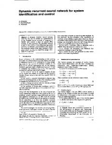
Fig. 1. Block diagram of feedback control system.

where y k ; u k ; H z 01 , and H z 01 are respectively the output, the input, the controlled plant model, and the multiplicative uncertainty. Hn z 01 is the known, controllable nominal model and Hn z 01 2 RH1 is proper and stable [25]. Also, z 01 is the delay operator, and the polynomials An z 01 ; Bn z 01 ; A z 01 ; B z 01 are respectively given as

() () ( )

( )

1 ( )

( ) ( ) ( )1 ( )1 ( ) n An (z 01 ) =1 + aj z 0j Bn (z 01 ) =

m i=0

1A (z01 ) =1 + 1B (z01 ) =

l

j =1

bi z 0i h j =1

(n m)

j z 0j

(5)

Fig. 2. Block diagram of the proposed method using one neural network.

(6)

B. Proposed Method

(7)

i z 0i

(h l): (8) i=0 Here, j ; i are unknown coefficients and l( n); h( m) are unknown orders of the polynomials 1A (z 01 ); 1B (z 01 ): The general block diagram of the feedback control system is shown in Fig. 1, where r(k) is the reference signal and e(k) = r(k) 0 y (k)

is the error between the reference signal and the plant output. First, consider a special case in which there is no uncertainty in the plant (1), that is H z 01 : The conventional feedback controller Gn z 01 for the nominal model Hn z 01 can be predesigned to produce a desirable response. The closed loop transfer function Fn z 01 is described by [26]

( ) ( )

1 ( )=0

( )

01 01 (9) = 1 +GnG(nz(z0)H1 )nH(nz(z0)1 ) : Next, consider the general case of 1H (z 01 ) 6= 0 with the controller G(z 01 ) for the plant H (z 01 ) defined as G(z 01 ) = Gn (z 01 )[1 + 1G (z 01 )] (10) 0 1 0 where 1G (z ) represents the modification of the controller G(z 1 ): Thus, the closed loop transfer function F (z 01 ) that consists of H (z 01 ) and G(z 01 ) can be given as 01 (z 01 ) F (z 01 ) = G(z 0)H (11) 1 + G(z 1 )H (z01 ) : If (9) and (10) are equivalent, the response of F (z 01 ) using H (z 01 ) and G(z 01 ) can agree with the desirable response [27].

^( )

()

01 1G (z01 ) = 0 1 +1H1(Hz(z0)1 ) : (12) However, since 1H (z 01 ) is unknown, the modified value 1G (z01 ) cannot be computed by (12). When 1H (z01 ) is 0over the admissible error’s range of the feedback controller Gn (z 1 ); the control system performance decreases, or yields a steady-state error, or even turns into unstable performance. In order to solve this control problem, in the next subsection we propose a new method that can identify the uncertainty H z 01 using a neural network and adaptively modify the control input from the feedback controller

1 ( )

()

()

() ^( )

( ) ()

(k) = y^(k) 0 y(k):

The output of the neural network input as

yNN (k)

(13) modifies the control

1u (k) = 0yNN (k):

(14)

Next, the working principle of the proposed method is explained. By using Fig. 1 and (10), the control input u k can be represented as

()

Fn (z 01 ) = y(k) r(k)

Carrying out an operation using (4) and (9)–(11), we can obtain the following transformation for this equivalence:

Gn (z 01 ):

Fig. 2 shows the block diagram of the proposed method in this paper. The output y k of the identification model is a sum of the output of the nominal model yn k and the identified output yid k that is the output of the neural network yNN k passed through the nominal model Hn z 01 : The neural network is trained using the identified error k between the model’s output y k and the plant’s output y k

()

u(k) = Gn (z 01 )[1 + 1G (z 01 )]e(k) = un (k) + 1u (k) un (k) = Gn (z 01 )e(k) 1u (k) =1G (z01 )un (k)

(15) (16) (17)

1()

where un k and u k are the nominal control input and the modification, respectively. Also, from (1) and (2) the output y k becomes

1()

() y(k) = Hn (z 01 )[1 + 1H (z 01 )]u(k) = yn (k) + Hn (z01 )1y (k) yn (k) = Hn (z 01 )u(k) 1y (k) =1H (z01 )u(k)

where y k is the uncertain output via the uncertainty Substituting (15), (17) into (20), we have

(18) (19) (20)

1H (z01 ):

1y (k) =1H (z01 )[un (k)+ 1u (k)] =1H (z01 )[1 + 1G (z01 )]un(k): By (17) and (22), the modification 1u (k) can be rewritten as 01 1u (k) = 1H (z011 )[1G (+z 1)G (z01 )] 1y (k):

(21)

(22)

Substituting (12) into (22), we obtain the following relation between

1u (k) and the uncertain output 1y (k): 1u (k) = 01y (k):

(23)

498


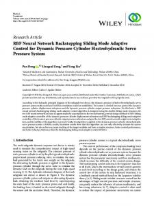
Fig. 3. Neural network used in the proposed method. Fig. 4. Sigmoid function used in the neural network.

On the other hand, by Fig. 2, (13) and (18), the identified error k can be given as

(

)

(k) =[Hn (z01 )yNN (k) 0 yn (k)] 0 [Hn (z01 )1y (k) + yn (k)] = Hn (z01 )[yNN (k) 0 1y (k)]:

()

( )

yNN (k) = 1y (k):

(25)

We can see that the output of the plant under the proposed method can agree with the desirable response using (14). As a result, the proposed method can adaptively control a class of plants with linear uncertainty given as (1)–(8) using the neural network. The proposed control system is designed to cancel out the effects of the second term in the right side of (18). Therefore, it should be noted that if the output y k can be decomposed as (18) and the uncertainty y k can be identified by learning of the neural network, the proposed method is also valid for nonlinear uncertainties included in y k : The effectiveness of the proposed method to the nonlinear uncertainties included in the plant will be verified in Sections III and IV. The next subsection explains how the modification u k in (14) can be realized using the neural network.

1() 1()

1()

C. Neural Network Model The multilayer neural network used in this paper is shown in Fig. 3. The numbers of units in the input layer and the hidden layer are N and M; respectively. The number of units of the output layer is one. In Fig. 3, wij k represents the weight that connects the unit j in the input layer and the unit i in the hidden layer; vi k represents the weight that connects the unit i in the hidden layer and the output unit; W k 2 > 0 = sup jHn (e0j!T )j 0! 1 % kQ k

kQ(k)k1 = sup

0kk

( )g

fQ k

(38) (39) (40)

()

where kL is the learning time, T is the sampling period, fQ k g (hereafter, abbreviated as k is the maximum singular value of the matrix Q k 2 0:01 for STNC, > 0:03 for FNAC and > 0:1 for PNAC), the control system became unstable and the neural network learning could not be converged. On the other hand, the proposed method always achieved stable learning of the neural network and adaptive control for the range 3:0: V. CONCLUSION In this paper, the new neural adaptive control method that can regulate the control input and identify the controlled plant with linear and nonlinear uncertainties by using only one neural network has been proposed. The working principle of the proposed method was explained and the sufficient condition of the local asymptotic stability near the optimal weight’s set was derived. Computer simulations were

504


W (k + 1) W (k) 0 (k)H n (z 01 ) 2 (k)V (k)U TIN (k): (56) The diagonal elements of the matrices

1 (k)

and

2 (k)

are

j!1ii (k)j M1 ; j!2ii (k)j M2 where M1 ; M2 are constants, since

() ()

the sigmoid function is of the tanh function. Therefore, 1 k ; 2 k are bounded matrices. By (55) and (56), assuming the identified error to be sufficiently small, we get VT k W k

( + 1) ( + 1) = [V T (k) 0 (k)H n (z01 )U TIN (k)W T (k) 1 (k)] 1 [W (k) 0 (k)H n (z01 ) 2 (k)V (k)U TIN (k)] V T (k)W (k) 0 (k)H n (z01 ) 1 [U TIN (k)W T (k) 1 (k)W (k) + V T (k) 2 (k)V (k)U TIN (k)]:

(a)

(57)

Substituting (34) into the parameter error (57) yields VT k W k

( + 1) ( + 1) V T (k)W (k) 0 H H n (z 01 )'T (k)U IN (k)H n (z 01 ) 1 [U TIN (k)W T (k) 1 (k)W (k) + V T (k) 2 (k)V (k)U TIN (k)] (58) = V T (k)W (k) 0 Hn (z01 )'T (k)Q(k):

(b)

Then substituting (58) into (35) yields 'T k %VV T k W

( + 1) = ( + 1) (k + 1) 0 T = 'T (k)[0 0 %HH n (z01 )Q(k)]

where 0 2 %kH n z01 Q k QT k k1 : (62)

( )+ ( ) ( ) () () Defining Q(k) to be a positive semi-definite matrix yields [43] kQ(k) + QT (k)k1 = kQ(k)k1 + kQT (k)k1 =2kQ(k)k1: (63) Finally, (62) can be represented as

2kQ(k)k1 > % fkQ(k)k1g2 that is

V (k + 1) V (k) 0 (k)H n (z 01 ) 1 (k)W (k)U IN (k) (55)

(60)

When the learning rate satisfies to the following expression Q k QT k 0 %H H n z 01 Q k QT k > (61)

APPENDIX Near the optimal set of the weights, the updating weight rules (29), (30) with the sigmoid function can be approximated as follows:

19 can

19 = 9(k + 1) 0 9(k) = 'T (k)[0 0 %HH n (z01 )Q(k)] 1 [0 0 %H H n (z 01 )QT (k)]'(k) 0 'T (k)'(k) = 0%HH n (z01 )'T (k)[Q(k) + QT (k) 0 %H H n (z 01 )Q(k)QT (k)]'(k):

(c)

performed to the plant with linear and nonlinear uncertainties, so that the effectiveness and asymptotic stability of the proposed method were clearly confirmed. Also the proposed method was applied to the torque control of a flexible beam in contact with the external environment. Even though the dynamic characteristics of the flexible beam were largely varied, the precise control was realized in the experiment. The comparison of the experimental results under the proposed method and other neural adaptive control methods was done in order to show the distinctive feature of the proposed method. In order to improve the performance of the controlled plant using the neural network, this paper have concentrated on the control structure of the controlled plant. The other way to improve the control performance is to revise the neural network model itself. In the future, we plan to improve the learning speed of the neural network and extend the proposed method to a general nonlinear plant and a multivariable system.

(59)

2

% kQ(k)k1

>>0

(64)

(65)

where

=

sup jH n (e0j!T )j:

0! 1

(66)


REFERENCES [1] K. S. Narendra and K. Parthasarathy, “Identification and control of dynamical systems using neural networks,” IEEE Trans. Neural Networks, vol. 1, no. 2, pp. 4–27, 1990. [2] F.-C. Chen and H. K. Khalil, “Adaptive control of nonlinear systems using neural networks,” Int. J. Contr., vol. 55, no. 6, pp. 1299–1317, 1992. [3] C.-C. Liu and F.-C. Chen, “Adaptive control of nonlinear continuoustime systems using neural networks–general relative degree and mimo cases,” Int. J. Contr., vol. 58, no. 2, pp. 317–335, 1993. [4] F.-C. Chen and C.-C. Liu, “Adaptively controlling nonlinear continuoustime systems using multilayer neural networks,” IEEE Trans. Automat. Contr., vol. 39, no. 6, pp. 1306–1310, 1994. [5] F.-C. Chen and H. K. Khalil, “Adaptive control of a class of nonlinear discrete-time systems using neural networks,” IEEE Trans. Automat. Contr., vol. 40, no. 5, pp. 791–801, 1995. [6] F. L. Lewis, K. Liu, and A. Yesildirek, “Neural net robot controller with guaranteed tracking performance,” IEEE Trans. Neural Networks, vol. 6, no. 3, pp. 703–715, 1995. [7] S. Jagannathan and F. L. Lewis, “Multilayer discrete-time neural-net controller with guaranteed performance,” IEEE Trans. Neural Networks, vol. 7, no. 1, pp. 107–130, 1996. [8] F. L. Lewis, A. Yesildirek, and K. Liu, “Multilayer neural-net robot controller with guaranteed tracking performance,” IEEE Trans. Neural Networks, vol. 7, no. 2, pp. 388–399, 1996. [9] T. Yabuta and T. Yamada, “Neural network controller characteristics with regard to adaptive control,” IEEE Trans. Syst., Man, Cybern., vol. 22, no. 1, pp. 170–176, 1992. [10] T. Yamada and T. Yabuta, “Some remarks on characteristics of direct neuro-controller with regard to adaptive control,” Trans. Soc. Instrum. Contr. Eng., vol. 27, no. 4, pp. 784–791, 1991. [11] L. G. Kraft, III, and D. P. Campagna, “A summary comparison of cmac neural network and traditional adaptive control systems,” in Neural Networks for Control, W. T. Miller, R. S. Sutton, and P. J. Werbos, Eds. Cambridge, MA: MIT Press, 1990. [12] N. Sadegh, “A perceptron network for functional identification and control of nonlinear systems,” IEEE Trans. Neural Networks, vol. 4, no. 6, pp. 982–988, 1993. [13] R. Carelli, E. F. Camacho, and D. Patino, “A neural network based feedforward adaptive controller for robots,” IEEE Trans. Syst., Man, Cybern., vol. 25, pp. 1281–1288, May 1995. [14] S. Akhyar and S. Omatsu, “Self-tuning pid control by neural networks,” in Proc. Int. Joint Conf. Neural Networks, 1993, pp. 2749–2752. [15] M. Khalid, S.Omatu, and R. Yusof, “Temperature regulation with neural networks and alternative control schemes,” IEEE Trans. Neural Networks, vol. 6, no. 3, pp. 572–582, 1995. [16] M. Kawato, Y. Uno, M. Isobe, and R. Suzuki, “A hierarchical model for voluntary movement and its application to robotics,” IEEE Contr. Syst. Mag., vol. 8, no. 2, pp. 8–16, 1988. [17] Y. Iiguni, H. Sakai, and H. Tokumaru, “A nonlinear regulator design in the presence of system uncertainties using multilayered neural network,” IEEE Trans. Neural Networks, vol. 2, no. 4, pp. 410–417, 1991. [18] C. Ku and K. Y. Lee, “Diagonal recurrent neural networks for dynamic systems control,” IEEE Trans. Neural Networks, vol. 6, no. 1, pp. 144–156, 1995. [19] M. M. Polycarpou and A. J. Helmicki, “Automated fault detection and accommodation: A learning systems approach,” IEEE Trans. Syst., Man, Cybern., vol. 25, pp. 1447–1458, Feb. 1995. [20] G. A. Rovithakis and M. A. Christodoulou, “Direct adaptive regulation of unknown nonlinear dynamical systems via dynamic neural networks,” IEEE Trans. Syst., Man, Cybern., vol. 25, pp. 1578–1594, Dec. 1995. [21] A. U. Levin and K. S. Narendra, “Control of nonlinear dynamical systems using neural networks–part ii: Observability, identification, and control,” IEEE Trans. Neural Networks, vol. 7, no. 1, pp. 30–42, 1996. [22] K. Takahashi, “Neural-network-based learning control applied to a single-link flexible arm,” in Proc. 2nd Int. Conf. Motion Vibration Control, 1994, pp. 811–816. [23] G. A. Rovithakis and M. A. Christodoulou, “Adaptive control of unknown plants using dynamical neural networks,” IEEE Trans. Syst., Man, Cybern., vol. 24, pp. 400–412, Mar. 1994. [24] M. A. Kaashoek, J. H. van Schuppen, and A. C. M. Ran, Robust Control of Linear Systems and Nonlinear Control. Boston, MA: Birkh¨auser, 1990. Control Theory. New York: Springer[25] B. A. Francis, A Course in Verlag, 1987.

H1

505

˚ o and B. Wittenmark, Adaptive Control. Norwell, MA: [26] K. J. Astr¨ Addison-Wesley, 1989. [27] T. Kailath, Linear Systems. Englewood Cliffs, NJ: Prentice-Hall, 1980. [28] D. E. Rumelhart, G. E. Hinton, and R. J. Williams, “Learning representations by error propagation,” in Parallel Distributed Processing, D. E. Rumelhart, J. L. McClelland, and PDP Research Group, Eds. Cambridge, MA: MIT Press, 1986, vol. 1, pp. 318–362. [29] G. Cybenko, “Approximation by superposition of a sigmoidel function,” in Artificial Neural Networks: Concepts and Theory, P. Mehra and B. W. Wah, Eds. Los Alamitos, CA: IEEE Comput. Soc. Press, 1992, pp. 488–499. [30] K. Funahashi, “On the approximate realization of continuous mappings by neural networks,” Neural Networks, vol. 2, pp. 183–192, 1989. [31] R. N. Clark, Control System Dynamic. Cambridge, U.K.: Cambridge Univ. Press, 1996. [32] M. Kaneko, “Active antenna,” in Proc. IEEE Int. Conf. Robotics Automation, 1994, pp. 2665–2671. [33] M. Kaneko, N. Kanayama, and T. Tsuji, “3-D active antenna for contact sensing,” in Proc. IEEE Int. Conf. Robotics Automation, 1995, vol. 1, pp. 1113–1119. [34] N. Ueno, M. Kaneko, and M. Svinin, “Theoretical and experimental investigation on dynamic active antenna,” in Proc. IEEE Int. Conf. Robotics Automation, vol. 3, pp. 3557–3563, 1996. [35] T. Fukuda, N. Kitamura, and K. Tanie, “Adaptive force control in robot manipulation with consideration of characteristics of objects,” Trans. Jpn. Soc. Mech. Eng., vol. 53, no. 487, pp. 726–730, 1987 (in Japanese). [36] T. Fukuda and A. Arakawa, “Control of flexible robotic arms,” Trans. Jpn. Soc. Mech. Eng., vol. 53, no. 488, pp. 954–961, 1987 (in Japanese). [37] M. Tokita and T. Fukuda, “Force control of robotic manipulator using neural network,” J. Robot. Soc. Jpn., vol. 14, no. 1, pp. 75–82, 1996 (in Japanese). [38] T. Yamada and T. Yabuta, “Nonlinear neural network controller for dynamic systems,” in Proc. 16th Annu. Conf. IEEE Industrial Electronics Soc., 1990, pp. 1244–1249. [39] E. Rijanto, A. Moran, T. Kurihara, and M. Hayase, “Robust tracking control of flexible arm using inverse dynamics method,” in Proc. 4th Int. Workshop Advanced Motion Control, 1996, pp. 669–674. [40] J. Lu, M. Shafiq, and T. Yahagi, “Vibration control of flexible robotic arms using robust model matching control,” in Proc. 4th Int. Workshop Advanced Motion Control, 1996, pp. 663–668. [41] K. S. Narendra and A. M. Annaswamy, Stable Adaptive Systems. Englewood Cliffs, NJ: Prentice-Hall, 1989. [42] W. T. Miller, R. S. Sutton, and P. J. Werbos, Neural Networks for Control. Cambridge, MA: MIT Press, 1990. [43] A. Weinmann, Uncertain Models and Robust Control. New York: Springer-Verlag, 1991.