181
IJCSS, Vol.1, No.2, 2000
A NEURAL NETWORK ROBUST CONTROLLER FOR REAL-TIME CONTROL OF INDUCTION MOTOR Daohang Sha Centre for Engineering Research, Technikon Natal, P.O.Box 953, Durban 4000, South Africa e-mail:
[email protected]
Accepted in the Þnal form: 15 November, 2000
Abstract. A neural network robust controller (NNRC) to enhance the robustness of the conventional feedback controller is proposed in this paper. The control system consists of an optimal conventional feedback controller and a neural network robust controller in parallel to the controlled system. The optimal controller is used to guarantee the stability of the whole control system and present the optimal tracking performance to the reference input signal. To overcome the uncertainties included in the plant, a neural network robust controller with an on-line learning algorithm is added to the conventional optimal controller for the identiÞcation of uncertainties and adaptive modiÞed control at the same time. The new controller has increased robustness with regard to parameter variations. The new controller also exhibits very good disturbance rejection property. Simulation experiments and real-time control are made to illustrate the quality and robustness of control achieved for the induction motor system.
Keywords: Neural networks, robust control, real-time control, induction motor
1
INTRODUCTION
Applications of the neural network to adaptive control of nonlinear systems have been intensively conducted in recent years. For example, Narendra and Parthasarathy [19] introduced multilayer neural networks for identiÞcation and adaptive control of nonlinear systems. A number of studies such as [6]-[9] for adaptive control of unknown feedback linearization systems and [16], [17] for achieving guaranteed performance of the neural net controller have been reported. This is due to the fact that the neural network has excellent capabilities of nonlinear mapping, learning ability, and parallel computations. Most of the proposed adaptive control methods using single neural networks can be classiÞed into four types: the direct neural adaptive control [27], [28], the parallel neural control [23], the feedforward neural adaptive control [5], and the self-tuning neural adaptive control [1], [13]. Yabuta and Yamada [27] proposed the direct neural adaptive control that replaces a conventional feedback controller with a neural network. Also, they discussed the stability of the linear discrete-time singleinput-single-output (SISO) plant[28]. Although their method is quite simple and can be applied to various feedback control systems, the uncertainty of the controlled plant cannot be identiÞed and some parameters included in the neural network is quite difficult to be set. On the other hand, as a parallel neural network adaptive control, Sadegh [23] presented an adaptive controller based on the neural network arranged in parallel to a conventional feedback controller. Their idea is to compensate the
182
IJCSS, Vol.1, No.2, 2000
control input computed from the conventional feedback controller for canceling the effect of the plant uncertainties. Also, Carelli et al. [5] proposed an adaptive controller using feedback error learning [12]. The neural network can gradually modify the control input from a conventional feedback controller and can Þnally take the place of the conventional feedback controller. Moreover, Akhyar and Omatsu [1] and Khalid et al. [13] presented a self-tuning controller that uses a set of neural networks for regulating the gains of the conventional feedback controller in order to improve the performance of the control system. Their methods could maintain stability of the adaptive control system through the function of the conventional feedback controller. Tsuji et al. [26] uses only a single neural network for both control and identiÞcation. In this method, an identiÞcation model is composed of a neural network and a linear nominal model which is approximated for the controlled plant. The neural network can identify the uncertainties included in the controlled plant and can adaptively modify the control input computed from a predesigned conventional feedback controller at the same time. For all of the methods presented above using single neural network, however, even if the adaptive controller of the controlled plant can be obtained by neural network learning, the uncertainty included in the controlled plant cannot be expressed explicitly. When the forward model for the controlled plant is necessary, the controlled plant must be identiÞed again by using other identiÞcation techniques. Besides, many of these methods may require long learning time or result in instability in some practical applications, where there are uncertainties between the input to the controlled plant and the error signal required for learning. Another approach to the neural adaptive control is to utilize multiple neural networks [10], [14], [15], [19], [20], [21], and [22]. In this approach, one neural network is dedicated to the forward model for identifying the uncertainties of the controlled plant and the other neural networks may compensate for the effect of the uncertainties based on the trained forward model. However, multiple neural networks must be trained and stability of this approach is quite difficult to assure. This paper adopts single neural networks added to the conventional optimal controller scheme. One advantage of this scheme is that the optimal controller is used to guarantee the stability of whole control systems and can present the optimal tracking performance to the reference input signal, while a neural network robust controller with on-line learning algorithm can signiÞcantly enhance the robustness of the optimal controller without affecting its tracking performance. To verify the effectiveness of this approach, it is applied to the speed control of induction motor subjected to parameter variation and unknown external disturbances. Simulations and experiments are used to evaluate the control system performance and comparison is made to the control effects obtained by a optimized PI controller. The results achieved show that the proposed NNRC has much better robustness than the optimally tuned PI controller.
2
NEURAL NETWORK ROBUST CONTROLLER DESIGN
In practice, there are always non-linearities and uncertainties caused by parameter variation, external disturbances or unmodelled dynamics, or the plant model for whatever reason is not completely known (see [4], [18]). To overcome these the unknown uncertainties included in the plant, we need an additional robust controller to the conventional feedback controller. To formulate the robust controller, let us discuss these uncertainties Þrstly.
2.1
Uncertainty of Controlled System
Let us consider a controlled plant with a multiplicative uncertainty described by y(k + 1) = H(z −1 )u(k), H(z −1 ) = Hn (z −1 )[1 + ∆H(z −1 )],
(1) (2)
where y(k + 1), u(k), H(z −1 ), and ∆H(z −1 ) are respectively the output, the input, the controlled plant model, and the multiplicative uncertainty. Hn (z −1 ) is the known, controllable nominal model.
183
IJCSS, Vol.1, No.2, 2000
The general block diagram of the feedback control system is shown in Fig.1. It consists of an optimal conventional feedback controller and a neural network robust controller in parallel to the controlled system. The optimal controller is used to guarantee the stability of the whole control system and present the optimal tracking performance to the reference input signal. To overcome the uncertainties included in the plant, a neural network robust controller with an on-line learning algorithm is added to the conventional optimal controller for the identiÞcation of uncertainties and adaptive modiÞed control at the same time. First, consider a special case in which there is no uncertainty in the plant (1), that is ∆H(z −1 ) = 0. The conventional feedback controller Gn (z −1 ) for the nominal model Hn (z −1 ) can be predesigned to produce a desirable response. The closed loop transfer function Fn (z −1 ) is described by Fn (z −1 ) =
Gn (z −1 )Hn (z −1 ) y(k) = , r(k) 1 + Gn (z −1 )Hn (z −1 )
(3)
where r(k) is the reference input. Next, Consider the general case of ∆H(z −1 ) 6= 0 with the controller G(z −1 ) for the plant H(z −1 ) deÞned as (4) G(z −1 ) = Gn (z −1 )[1 + ∆G(z −1 )] where ∆G(z −1 ) represents the modiÞcation of the controller G(z −1 ). Thus, the closed loop transfer function F (z −1 ) that consists of H(z −1 ) and G(z −1 ) can be given as F (z −1 ) =
G(z −1 )H(z −1 ) . 1 + G(z −1 )H(z −1 )
(5)
If (3) and (5) are equivalent, the response of F (z −1 ) using H(z −1 ) and G(z −1 ) can agree with the desirable response. Carrying out an operation using (2) and (3)-(5), we can obtain the following transformation for the equivalence: ∆G(z −1 ) = −
∆H(z −1 ) . 1 + ∆H(z −1 )
(6)
However, since ∆H(z −1 ) is unknown, the modiÞed value ∆G(z −1 ) cannot be computed by (6). When ∆H(z −1 ) is over the admissible error’s range of the feedback controller Gn (z −1 ), the control system performance decreases, or yields a steady-state error, or even turns into unstable performance. In order to solve this control problem, in the next subsection we propose a new method that can identify the uncertainty ∆H(z −1 ) using a neural network and adaptively modify the control input from the feedback controller Gn (z −1 ).
2.2
Neural Network Robust Controller
Fig. 1 shows the block diagram of the used method in this paper. The output yˆ(k + 1) of the identiÞcation method is a sum of the output of the nominal model yn (k + 1) and the identiÞed output yid (k + 1) that is the output of the neural network yNN (k + 1) passed through the nominal model Hn (z −1 ). The neural network is trained using the identiÞed error ε(k + 1) = y(k + 1) − yˆ(k + 1).
(7)
The output of the neural network yN N (k + 1) modiÞes the control input as ∆u(k) = −yNN (k + 1).
(8)
By using Fig.1 and (4), the control input u(k) can be represented as u(k) = Gn (z −1 )[1 + ∆G(z −1 )]e(k) = un (k) + ∆u(k), −1
un (k) = Gn (z )e(k), ∆u(k) = ∆G(z −1 )un (k),
(9) (10) (11)
184
IJCSS, Vol.1, No.2, 2000
NN Robust Controller ϕ
TDL
W
v f (ϕ )
+
ynn(k + 1)
TDL
Hn ( z − 1 ) r(k) +
e(k)
-
yn (k + 1)
Gn (z−1) NSMC
-1
∆u(k)
Hn ( z − 1 ) yid (k + 1)
On-line Updating
+
+
yˆ (k + 1) -
+
++ u(k)
ε (k + 1)
H(z−1)
y(k + 1)
Nonlinear Plant
Figure 1: Scheme of Neural Network Robust Controller where un (k) and ∆u(k) are the nominal control input and the modiÞcation, respectively. Also, from (1) and (2) the output y(k + 1) becomes y(k + 1) = Hn (z −1 )[1 + ∆H(z −1 )]u(k) = yn (k + 1) + Hn (z −1 )∆y(k + 1), yn (k + 1) = Hn (z −1 )u(k), ∆y(k + 1) = ∆H(z −1 )u(k),
(12) (13) (14)
where ∆y(k +1) is the uncertain output via the uncertainty ∆H(z −1 ). Substituting (9), (11) into (14), we have (15) ∆y(k + 1) = ∆H(z −1 )[un (k) + ∆u(k)] = ∆H(z −1 )[1 + ∆G(z −1 )]un (k). By (11) and (15), the modiÞcation ∆u(k) can be rewritten as ∆u(k) =
∆G(z −1 ) ∆y(k + 1). ∆H(z −1 )[1 + ∆G(z −1 )]
(16)
Substituting (6) into (16), we obtain the following relation between ∆u(k) and the uncertain output ∆y(k + 1) : ∆u(k) = −∆y(k + 1). On the other hand, by Fig. 1, (7) and (12), the identiÞed error ε(k + 1) can be given as ε(k + 1) = y(k + 1) − [Hn (z −1 )yNN (k + 1) + yn (k + 1)] = [yn (k + 1) + Hn (z −1 )∆y(k + 1)] − [Hn (z −1 )yNN (k + 1) + yn (k + 1)] = Hn (z −1 )[∆y(k + 1) − yNN (k + 1)].
(17)
If the neural network is well trained, we can expect that ε(k + 1) Þnally becomes zero in (17). Since Hn (z −1 ) is the nominal model and is not identically zero, we can have yNN (k + 1) = ∆y(k + 1). We can see that the output of the plant under the proposed method can agree with the desirable response using (8). As a result, the proposed method can adaptively control a class of plants with linear uncertainty given as (2) using the neural network. The proposed control system is designed to cancel out the effects of the second term in the right side of (12). Therefore, it should be noted that if
185
IJCSS, Vol.1, No.2, 2000
the output y(k + 1) can be decomposed as (12) and the uncertainty can be identiÞed by learning of the neural network, the proposed method is also valid for nonlinear uncertainties included in ∆y(k + 1). So the single neural network can achieve not only the identiÞcation of the uncertainties but also the control of the plant.
2.3
On-line Learning of Neural Network
Consider a three layer forward neural network as a robust controller yN N =
HN X i=1
P
s
IN X
j=1
wij ϕj + wi0 vi + v0 =
HN X i=0
s
IN X
j=0
wij ϕj vi =
HN X
s (neti ) vi
(18)
i=0
where neti = IN j=0 wij ϕj is the output of ith hidden node with ϕ0 ≡ 1, for i = 0, 1, · · ·, HN, and with s (net0 ) ≡ 1. Here ϕj , j = 1, · · ·, IN, are the inputs of the neural network, yNN is the output of the neural network, wij , i = 1, · · ·, HN , j = 1, · · ·, IN, are the weights from input layer to hidden layer, wi0 , i = 1, · · ·, HN, are the biases (or threshold) of hidden nodes, vi , i = 1, · · ·, HN, are the weights from hidden layer to output layer, v0 is the bias of output node, IN is number of nodes of input layer, HN is the number of nodes of hidden layer, s is the active function of nodes for hidden layer and output layer. Further, (18) can be rewritten as yNN (k + 1) = vT S(W ϕ), where ϕ= v=
W = S(W ϕ) =
h
h
h
ϕ0 ϕ1 · · · ϕIN v0 v1 · · · vHN
w10 w11 w20 w21 ··· ··· wHN0 wHN1
iT
iT
∈ R(IN+1)×1 , ∈ R(HN+1)×1 ,
· · · w1IN · · · w2IN ··· ··· · · · wHN IN
∈ RHN×(IN+1) ,
s(net0 ) s(net1 ) · · · s(netHN )
iT
∈ R(HN+1)×1 .
the active function for non-linear nodes is a symmetric hyperbolic tangent function, i.e. s(x) = tanh( µx ), and its derivative is s0 (x) = µ1 [1−s2 (x)], .where µ0 is the shape factor of the active function. 0 0 Let us deÞne the error function for on-line learning as 1 1 J(k) = ε2 (k) = [y(k) − yˆ(k)]2 , 2 2 where yˆ(k) = Hn (z −1 )yNN (k + 1) + yn (k + 1). By applying the gradient descent method to J, one obtains the on-line updating of weights of the neural network for robust controller is as follows ∆v = η
∂yid (k) ¯0 ∂yid (k) S(W ϕ)ε(k), ∆W = η S (W ϕ)¯ vϕT ε(k), ∂yNN (k) ∂yNN (k)
where η is the learning rate of a small positive constant,
∂yid (k) ∂yNN (k)
=
of nominal model of controlled plant which can be approximated by v¯ =
h
S¯0 (W x) = diag
h
v1 ... vHN
iT
∂yn (k) ∂u(k) is ∆yn (k) ∆u(k) ,
∈ RHN×1 ,
s0 (net1 ) s0 (net2 ) ... s0 (netHN )
i
,
the sensitivity function
186
IJCSS, Vol.1, No.2, 2000
1
1/170
Load
Additive Noise
Sensor Noise
Proportional 1
2 0.01s+1 control Saturation Rate Limiter Unmodelling input dynamic
Multiplicative noise 170
1
0.065s+1 Induction motor
output speed
Transport Delay
Figure 2: Simulation model for the induction motor ∂s(neti ) , for i = 1, ..., HN. For speeding up the learning process and avoiding the ∂neti trouble to select the learning rate for the neural networks, a variable rate learning algorithm based on the gradient method is adopted, which is derived in the similar way proposed in [24] and [25], i.e. 0 < η(k) < 2ζ −1 (k), where and s0 (neti ) =
ζ(k) =
µ
∂yid (k) ∂yNN (k)
¶2 h
Note that here a little difference is that the term of
3
i
S T (W ϕ)S(W ϕ) + v¯T S¯0 (W ϕ)S¯0 (W ϕ)¯ vϕT ϕ . ∂yid (k) ∂yN N (k)
is added to the formula only.
SIMULATION EXPERIMENTS
The simulation experiments are performed to preliminarily investigate the control performance of the new controller. Simulation is based on the approximate model of the induction motor speed control system used for the real-time laboratory experiments. The structure of the simulation model for the induction motor and the associated components is shown in Fig. 2. The continuous transfer function of the motor speed system to be controlled is identiÞed from K Y (s) = e−Ls . Here, K = 170 rev. min−1 , τ = 0.01 sec, an on-line experiment as U(s) (τ s + 1)(T s + 1) T = 0.065 sec, and L = 0.02 sec, are the static gain, time constant, and dead time, respectively. The sampling time is chosen as Ts = 0.02 sec, so the time delay of this system is one step. We used only the Þrst order approximate model to represent the motor in simulation experiments, while the other part of the transfer function model is used to represent the unmodelled dynamics of the system. Also, both the additive and the multiplicative noise signals are added to the simulation model in an attempt to making it more realistic. Finally, an additional rate limiter and control limiter are added to the control system and used with both the optimized PI and NNRC controller. These components are added to prevent sudden large changes in the control signal. The rate limits are selected as ±50 V sec−1 , and the saturation values of the control limiter as 0 ÷ 5 V. The results for the PI+NNRC are shown simultaneously with the results obtained with the optimized PI controller. For the considered nominal operation mode of the induction motor, the PI controller is optimally tuned to minimize step type disturbances acting at the input to the induction motor with the rate limiter and control signal limiter active. The performance index function is taken as the integral (sum) absolute error (IAE) between the achieved motor response and the given reference input. The structure of neural network used in the NNRC is 4 × 5 × 1, i.e. there are four inputs and Þve hidden neurons; two inputs u(k) and u(k − 1) to the neural networks are from the control signals and two inputs y(k) and y(k − 1) are from the past outputs of the plant via TDL (Tapped Delay Line) blocks. Although the neural network used in NNRC has a on-line self-learning ability during the control, it still needs to be trained off-line; the reasons are that there are no enough time and no rich exciting signals for neural networks to learn in the simulation and real-time control showed in late.
187
IJCSS, Vol.1, No.2, 2000
setting point tracking (Fig. 3) disturbance rejection (Fig. 4) gain variation (Fig. 5)
Optimal PI PI+NNRC Optimal PI PI+NNRC Optimal PI PI+NNRC
J(0.5, 2) 36.29 26.52 36.29 26.52 36.29 26.52
J(2, 3.5) 10.18 8.892 11.68 8.489 14.14 10.27
J(3.5, 5) 18.74 15.97 10.88 7.643 23.33 16.26
Table 1: Values of the cost function in characteristic time intervals Set point tracking 600
500
Motor output speed (rpm)
400 Input→
300
Optimal PI with NNRC
200
100
0
0
0.5
1
1.5
2
2.5 time(seconds)
3
3.5
4
4.5
5
Figure 3: Set-point tracking The parameters for PI controller are Kp = 0.5, Ki = 8. The velocity tracking, disturbance rejection and the (artiÞcial) gain variation simulation for the induction motor with PI+NNRC and PI control are given in Fig. 3, Fig. 4, and Fig. 5, respectively. The control signal for a disturbance rejection experiment is presented in Fig. 6. From these Þgures, one can observe that the better disturbance rejection performance and robustness under parameter variations can be achieved by using PI+NNRC proposed in this paper than compared to the pure optimized Pi controller. In order to assess the 1 Rb |e(t)| dt as a cost effectiveness of the PI+NNRC in a quantitative manner, we use J(a, b) = b−a a function. In the three time intervals corresponding to the response rise period (the initial transient, 0.5−2 sec.), the middle period (2−3.5 sec.), and the Þnal transient response period (the Þnal transient, 3.5 − 5 sec.), the cost function is calculated. The results are shown in Table 2. As can be observed, the PI+NNRC is the less tracking errors in disturbance rejection and gain variation as compared to the optimally tuned PI controller. However, it must be noted that the gain variation is not typical for the laboratory system used in the next section, and it is employed here only for the purpose of simulation with the aim to test the general robustness properties of the controllers.
188
IJCSS, Vol.1, No.2, 2000
Disturbance Rejection 600
500
Motor output speed (rpm)
400 Input→
Optimal PI with NNRC
300
200
100 ←Disturbance
0
0
0.5
1
1.5
2
2.5 time(seconds)
3
3.5
4
4.5
5
Figure 4: Simulation results for disturbance rejection
K=170→255→127.5, Gain Variation 600
500
Motor output speed (rpm)
400 Input→
300
200
Optimal PI with NNRC 100
0
0
0.5
1
1.5
2
2.5 time(seconds)
3
3.5
4
4.5
5
Figure 5: Simulation results for the artiÞcial gain variation of plant
189
IJCSS, Vol.1, No.2, 2000
Control signals for disturbance rejection 4
3.5
Control Signal: u(k) [Volt]
3
2.5
2
Optimal PI with NNRC
1.5
1
0.5
0
0
0.5
1
1.5
2
2.5 3 Time(seconds)
3.5
4
4.5
5
Figure 6: Control signals for disturbance rejection Control algorithms DSMC PID dSPACE software TRACE COCKPIT
D/A PC
M Optical Encoder
DS1102 Inverter D/A
M Inverter
Load motor
Figure 7: Induction motor speed real-time control system
4 4.1
REAL-TIME LABORATORY EXPERIMENTS Experimental Device
The experimental device used is the real-time motor speed control system shown in Fig. 7. The experimental system consists of two motors, one of which is the driving motor, and the other serves as the load. The shafts of the motors are connected via a chain transmission. The characteristics of the induction motors are as follows: 230V, 0.45kW, 50Hz, 1475rpm. The inverters of both motors (YASKAWA, VS mini, 200V single phase, 0.2kW) are controlled by the PC, providing a possibility for full control for experimental purposes of both the driving motor and the load motor. The interfacing is made via a dSPACE DSP1102 control board. This board is suitable for control and it is based on the ßoating-point DSP TMS320C31/60 MHz processor. It supports most of the simulation Þles that are built in the Matlab/Simulink environment. The Matlab/Simulink control model can be converted and downloaded to the DSP1102, and then it can work independently of the Matlab/Simulink environment. During the real-time operation of the
190
IJCSS, Vol.1, No.2, 2000
Disturbance rejection (Fig. 9) Gain variation (Fig. 10)
Properties undershoot (rpm) recovery time (sec) overshoot (rpm) recovery time (sec) overshoot (rpm) recovery time (sec) undershoot (rpm) recovery time (sec)
Optimal PI 75 0.45 88 0.55 128 0.55 155 1.05
with NNRC 57 0.4 65 0.4 128 0.25 110 0.7
Table 2: Comparison of the performance index of experimental results: the recovery time is measured in the case when the tracking error is between 390 and 410 rpm. control algorithm, the supervision and capturing of the important data can be done by the TRACE and COCKPIT software provided with the DSP board. DSP1102 has four input A/D channels (2 × 16 bit×4µs, 2×12 bit×1.25µs); four output D/A channels (12 bit×4µs); a complete subsystem for digital I/O signals, including 6 channels, PWM generation and bit-selectable 16 digital I/O lines; and two parallel incremental encoder channels with a 24 bit position counter. In our experiments, we use two D/A channels for control and one incremental encoder channel for speed measurements. The optical encoder used for measuring the motor speed is TRD-J600-RZ with a basic resolution of 600 pulses per revolution. By making use of the 4-times frequency technology in the DSP1102 counter channel, we can get a resolution of up to 2400 pulses per revolution. Due to the simplicity of the PI+NNRC algorithm, the time required for the execution of all of the operations during successive sampling is much less than 0.01 sec. To implement the PI+NNRC we only need to measure the speed of the induction motor. At each sampling interval the DSP board receives the actual position indicated by the encoder, from which the motor speed is calculated; the position signal has also been Þltered using a Þrst-order digital Þlter; then the controller is run.
4.2
Results of Real-time Experiments
In this subsection, we present experimental results that demonstrate effective performance of the proposed PI+NNRC. We present comparative results using the PI controller which is optimally tuned for disturbance rejection and PI+NNRC. The parameters for the PI+NNRC and PI controllers are the same as the ones used for the previous simulation experiments. The experimental results for the set-point tracking, disturbance rejection and the (artiÞcial) parameter variation are plotted in Fig. 8, Fig. 9, and Fig. 10, respectively. A comparison of the performance index is shown in Table 2. From these Þgures and the Table 2, it is clear that the NNRC which we propose is much more efficient in terms of disturbance rejection and also more robust under the artiÞcial parameter variation of the plant, than the optimally tuned PI controller. Tracking properties remain virtually the same for all three controllers. The non-smooth characteristics of the NNRC control signal is a consequence of the signiÞcant level of measurement noise caused by the chain transmission between the motors. This indicates that additional Þltering may be necessary in sensitive applications. The overall conclusion is the PI+NNRC outperforms pure optimized PI controller.
5
CONCLUSIONS
A new PI+NNRC control structure is proposed in this paper. It consists of an optimal conventional feedback controller and a neural network robust controller in parallel to the controlled system. The
191
IJCSS, Vol.1, No.2, 2000
Set point tracking 600
500
Motor output speed (rpm)
400
300
200
Optimal PI PI + NNRC 100
0
0
1
2
3 4 Time (seconds)
5
6
7
Figure 8: Experimental results for set-point tracking
Disturbance Rejection 550
Motor output speed (rpm)
500
450
400
350
Optimal PI PI + NNRC 300
250
2
2.5
3
3.5
4
4.5 5 Time (seconds)
5.5
6
6.5
Figure 9: Experimental results for disturbance rejection
7
192
IJCSS, Vol.1, No.2, 2000
Gain variation 550
Optimal PI PI + NNRC
Motor output speed (rpm)
500
450
400
350
300
250
2
2.5
3
3.5
4
4.5 5 Time (seconds)
5.5
6
6.5
7
Figure 10: Experimental results for artiÞcial gain variation
control signal for disturbance rejection 4
Optimal PI PI + NNRC
3.5
Control signal (Volt)
3
2.5
2
1.5
1
0.5
0
2
2.5
3
3.5
4
4.5 5 Time (seconds)
5.5
6
6.5
7
Figure 11: Measured control signals for disturbance rejection in experiements
IJCSS, Vol.1, No.2, 2000
193
optimal controller is used to guarantee the stability of the whole control system and present the optimal tracking performance to the reference input signal. To overcome the uncertainties included in the plant, a neural network robust controller with an on-line learning algorithm is added to the conventional optimal controller for the identiÞcation of uncertainties and adaptive modiÞed control at the same time. Simulation experiments and real-time control in laboratory conditions using industrial devices are made to illustrate the quality and robustness of control achieved for the induction motor system. Results have shown that the new PI+NNRC structure proposed performs much better than the conventional (optimally tuned) PI controller with regard to the disturbance rejection, tracking, and (artiÞcial) parameter variations.
References [1] S. Akhyar, S. Omatsu, Self-tuning PID control by neural networks, in Proc. Int. Joint Conf. Neural Network, 1993, pp. 2749-2752. [2] B. Armstrong-Helouvry, P.Dupont, and C. Canudas de Wit, A survey of analysis tools and compensation methods for the control of machines with friction, Automatica, Vol.30, pp.10831138, 1994. [3] C. Canudas de Wit, H.Olsson, K. J. Astrom and P. Lischinsky, A new model for control of systems with friction, IEEE Trans. Automat. Contr., vol.40, no.3, pp.419-425, 1995. [4] C. Canudas de Wit and P. Lischinsky, Adaptive friction compesation with partially known dynamic friction model, Int. J. Adaptive Control and Signal Proceedings, Vol.11, pp.65-80, 1997. [5] R. Carelli, E. F. Camacho, and D. Patino, A neural network based feedforward adaptive controller for robots, IEEE Trans. Syst., Man, Cybern., Vol.25, pp.1281-1288, May 1995. [6] F.-C. Chen and H. K. Khalil, Adaptive control of nonlinear systems using neural networks, Int. J. Contr., Vol.55, No.6, pp.1299-1317, 1992. [7] C.-C. Lui, F.-C. Chen, Adaptive control of nonlinear continuous-time systems using neural networks-general relative degree and mimo cases, Int. J. Contr., Vol.58, No.2, pp.317-335, 1993. [8] F.-C. Chen, C.-C. Lui, Adaptively controlling nonlinear continuous-time systems using multilayer neural networks, IEEE Trans. Automat. Contr., Vol.39, No.6, pp.1306-1310, 1994. [9] F.-C. Chen and H. K. Khalil, Adaptive control of a class nonlinear discrete-time systems using neural networks, IEEE Trans. Automat. Contr., Vol.40, No.5, pp.791-801, 1995. [10] Y. Iiguni, H. Sakai, H.Tokumaru, A nonlinear regulator design in the presence of system uncertainties using multilayered neural network, IEEE Trans. Neural Networks, Vol.2, No.4, pp.410-417, 1991. [11] S. Jagannathan, F. L. Lewis, Mutilayer discrete-time neural-net controller with guranteed performance, IEEE Trans. Neural Networks, Vol.7, No.1, pp.107-130, 1996. [12] M. Kawato, Y. Uno, M. Isobe, and R. Suzuki, A hierarchical model for voluntary movement and its application to robotics, IEEE Contr. Syst. Mag., Vol.8, No.2, pp.8-16, 1988. [13] M. Khalid, S. Omatu, Tempreture regilation with neural networks and alternative control schemes, IEEE Trans. Neural Networks, Vol.6, No.3, pp.572-582, 1995. [14] C. Ku, K. Y. Lee, Diagonal recurrent neural networks for dynamic systems control, IEEE Trans. Neural Networks, Vol.6, No.1, pp.144-156, 1995.
194
IJCSS, Vol.1, No.2, 2000
[15] A. U. Levin, K. S. Narendra, Control of nonlinear dynamical systems using neurak networks - part II: Observability, identiÞcation, and control, IEEE Trans. Neural Networks, Vol.7, No.1, pp.30-42, 1996. [16] F. L. Lewis, K. Lui, and A. Yesildirek, Neural net robot controller with guranteed tracking performance, IEEE Trans. Neural Networks, Vol.6, No.3, pp.703-715, 1995. [17] F. L. Lewis, A. Yesildirek, K.Lui, Mutilayer neyral-net robot controller with guranteed tracking performance, IEEE Trans. Neural Networks, Vol.7, No.2, pp.388-399, 1996. [18] P. Lischinsky, C. Canudas-de-Wit, and Morel, Friction Compensation for an Industial Hydraulic Robot, IEEE Control Systems Magazine, VOl.19, No.1, pp.25-32, 1999. [19] K. S. Narendra, K. Parthasarathy, IdentiÞcation and control of dynamical systems using neural networks, IEEE Trans. Neural Networks, Vol.1, No.2, pp.4-27, 1990. [20] M. M. Ploycarpou, A. J. Helmicki, Automated fult detection and accommodation: A learning systems approach, IEEE Trans. Syst., Man, Cybern., Vol.25, pp.1447-1458, Feb. 1995. [21] G. A. Rovithakis, M. A. Christodoulou, Adaptive control of unknown plants using dynamical neural networks, IEEE Trans. Syst., Man, Cybern., Vol.24, pp.400-412, Mar. 1994. [22] G. A. Rovithakis, M. A. Christodoulou, Direct adaptive regulation of unknown nonlinear dynamical systems via dynamic neural networks, IEEE Trans. Syst., Man, Cybern., Vol.25, pp.1578-1594, Dec. 1995. [23] N. Sadegh, A perceptron network for functional identiÞcation and control of nonlinear systems, IEEE Trans. Neural Networks, Vol.4, No.6, pp.982-988, 1993. [24] D. Sha, V. B. Bajic, On-line Adaptive Learning Rate BP Algorithm for Multi-layer Feed-forward Neural Networks, Journal of Applied Computer Science, Vol.7, No.2, 67-82, 1999. [25] D. Sha, V. B. Bajic, On-line Hybrid Learning Algorithm for MLP in IdentiÞcation Problems, an International Journal of Computer & Electrical Engineering, in print [26] T. Tsuji, B. H. Xu, M. Kaneko, Adaptive Control and IdentiÞcation Using One Neural Network for a Class of Plants with Uncertainties, IEEE Transaction on Systems, Man, And Cybernetics, Part A: Systems and Humans, Vol. 28, No. 4, pp. 496-505, JULY 1998. [27] T. Yabuta, T. Yamada, Neural network controller characteristics with regard to adaptive control, IEEE Trans. Syst., Man, Cybern., Vol.22, No.1, pp.170-176, 1992. [28] T. Yamada, T. Yabuta, Some marks on characteristics of direct neuro-controller with regard to adaptive control, Trans. Soc. Instrum. Contr. Eng., Vol.27, No.4, pp.784-791, 1991.