In this paper, design of a nonlinear controller for a. Bioreactor Benchmark Problem is presented. The system under control simulates the dynamical behaviour.
NEURAL NETWORK ASSISTED NONLINEAR CONTROLLER FOR A BIOREACTOR Mehmet Önder Efe
Okyay Kaynak
Ender Abadoglu
Electrical & Electronic Eng. Dpt.
Electrical & Electronic Eng. Dpt.
Mathematics Dpt.
Bogazici University
Bogazici University
Bogazici University
Istanbul, 80815, Turkey
Istanbul, 80815, Turkey
Istanbul, 80815, Turkey
ABSTRACT In this paper, design of a nonlinear controller for a Bioreactor Benchmark Problem is presented. The system under control simulates the dynamical behaviour of a biochemical process. The process has a few state variables but controller design is highly involved due to the nonlinear behaviour of the process, existence of limit cycles in the uncontrolled dynamics and the inherent delays. The proposed controller is also nonlinear, proven to be stable in the sense of bounded input/bounded output and locally stabilizing in the sense of Lyapunov. Additionally, neural networks are utilized in the controller design. A neural network is trained to partially identify the process dynamics and the trained network is used in the closed-loop control system. An error analysis is given for the neuro-identifier assisted controller performance.
1. INTRODUCTION Chemical systems are often highly nonlinear and difficult to control. Nonlinearities may be intrinsic to the physics or the chemistry of a process or may arise through the close coupling of a number of simpler processes. In either case, complicated differential or difference equations of the system dynamics pose a challenging problem in the sense of mathematical tractability. This problem can somewhat be alleviated by using a simplified model, but a control approach designed on the basis of such a simplified model is unlikely to result in a satisfactory performance. A prime example is a bioreactor. The commonly used model for this process has few state variables but the controller design is highly involved due to the nonlinear characteristics of the process and the existence of limit cycles in the uncontrolled dynamics. Anderson and Miller [1] list this plant as a challenging control problem and Agrawal and Lim [2] give an analysis of various control schemes. In recent years tremendous advances have been made in technology and this has affected the practice of control engineering. With the advances in high speed
computing, it is now possible and economically feasible to use complex, model-based control paradigms in practical applications, using advanced strategies derived from adaptive, non-linear, and robust control theories. The problem of bioreactor control has also benefited from these developments and various novel (mainly adaptive) strategies have been reported [3], with the objective of maintaining the process output close to the desired value in the presence of various uncertainties, including external disturbances, time-varying parameters, and unmodeled dynamics. A recent survey and comparison of various control configurations can be found in [4]. A more recent tendency in process control is the blending of algorithmic techniques with other elements, such as logic, reasoning and heuristics. Such systems have come to be known as intelligent control systems [5-6]. A host of new control approaches are being used in this respect, based on fuzzy logic, neural networks, evolutionary computing and other techniques adapted from artificial intelligence. In demonstrating the feasibility and efficacy of such approaches in the control of nonlinear processes, bioreactor control has been taken as a case study by many authors [7-9], some has addressed the topic directly. For example Feldkamp and Puskorius [10] take the bioreactor benchmark problem set by Ungar [11] and apply dynamic gradient methods, using neural networks for identification and control. In the work of Gorinevsky [12], the same benchmark problem is treated using affine radial basis function network architecture. It is shown that a completely adaptive control of this stongly nonlinear system can be achieved with minimal a priori knowledge of its dynamics. In this paper, the well-known Bioreactor Benchmark Problem is analyzed. The problem involves two state variables. One of them represents the biological cell concentration, and the other one represents the nutrient concentration in a tank. The objective is to keep the concentration of biological cell concentration at a desired level. The system has one control input meaning that external pure water is supplied into the tank and the same amount of mixture is removed from the reactor tank. This
343
is to keep the volume constant throughout the normal operation of the system. The second section describes the problem in detail.
In the simulations, these equations are discretized by the use of first order approximation with ∆ = 0.01sec. In (1) and (2), β = 0.02 (growth rate parameter), γ = 0.48 (nutrient inhibition parameter). Controller inputs are the state variables and the command signal. The control interval is defined to be 50∆. The output of the controller is the flow rate u(t). The objective is to achieve and maintain a desired cell amount by altering the flow rate.
At the analysis level of the reactor dynamics, a special reference model and the philosophy that lies behind this specific choice are explained. By utilizing the wellknown Model Reference Control (MRC) technique, the structure of the controller (or the rule of control) is established. The third section dwells on MRC and its analysis, which constitute the basis of controller design. The fourth section explains how neural networks can be injected into the proposed rule of control. A brief explanation of neurocomputing is given and the partial identification scheme is scrutinised. The subsequent section is devoted to the error convergence analysis of the proposed control strategy. Finally the simulation results and conclusions are presented.
The bioreactor is a challenging control problem for several reasons. Although the task involves few variables and is easily simulated, its non-linearity makes it difficult to control [11]. For example, small changes in the values of the parameters can cause the bioreactor to become unstable. The issues of delay, non-linearity, instability and limit cycles can be studied with the bioreactor control problem. Additionally, significant delays exist between changes in flow rate and the response in cell concentration [11].
2. PLANT MODEL
3. MODEL REFERENCE CONTROL OF A BIOREACTOR
As is previously stated, the model used is in this paper for the bioreactor is the one set by Ungar [11] as a benchmark problem. The process is a tank containing water, nutrients, and biological cells as shown in Fig. 1. Nutrients and cells are introduced into the tank where the cells mix with nutrients. The number of cells c1(t) and the amount of nutrients c2(t) characterize the state of this process. The volume in the tank is maintained at a constant level by removing tank contents at a rate equal to the incoming rate which is denoted by u(t). This rate is called the flow rate and is the variable by which the bioreactor is controlled. The system therefore has only one control input, which is the externally supplied pure water. The bioreactor control problem is to maintain the amount of cells at a desired level. Continuous time equations of the plant dynamics are given by (1) and (2). c�1(t) = − c1(t)u(t) + c1(t)(1 − c 2 (t))e
c� 2(t) = − c 2(t)u(t)+c1(t)(1 − c2(t))e
c2(t)
γ
c2(t)
γ
1+ β 1 + β − c2(t)
Model reference control technique is applicable to a wide variety of linear and nonlinear systems. The strategy evaluates some control inputs so that the plant output tracks a stable reference model output. There are two approaches in the model reference control approach: direct adaptive control and indirect adaptive control. In this paper, the latter is employed and is illustrated in Fig. 2. Indirect adaptive control scheme utilizes the instantaneous tracking error, which is denoted by ec, in parameter updating. Several past control inputs and plant outputs are provided by tapped delay lines which are represented by TDL blocks and which functions at the rate of 50∆ for this application. The parameters of the controller are directly adjusted to reduce some norm of the output error [13].
(1)
Indirect adaptive control scheme employs an additional plant identification model which can provide information about the nonlinear components that appear in the actual plant dynamics. In this study, a feedforward neural network is used as the identifier. The identification can be carried out on-line or off-line. The strategy adopted here is the indirect control scheme with off-line identification of the plant dynamics.
(2)
The state variables c1(t) and c2(t) can take values between zero and one, the flow rate u(t) can take values between zero and two. In the benchmark problem, the stable state of the process is defined to be c1 = 0.1207, c2 = 0.8801, and u = 0.7500. The initial values of the state variables lie within plus or minus ten percent of the related stable state value and the initial value of each state variable is assumed to be uniformly distributed random variable over the above mentioned interval.
By introducing f(c1,c2) and g(c2) and dropping the time variable, the governing equations of the bioreactor can be written more compactly as given by (3) and (4), c�1 = − c1u + f(c1 ,c 2 )
344
(3)
(4)
c� 2 = − c 2 u + f(c1 ,c 2 )g(c 2 )
u=
where, the definitions of f and g are clear from (1) and (2).
(5)
c� 2 m (t) = − c 2 m (t) + g (c 2 m (t))r(t)
(6)
u (c1(t), c 2 (t), r(t)) =
A neural network architecture, in the sense of feedforward data processing, comprises three main parts. The first part is the input layer that distributes the input data to the processors in the next layer. The second part is comprised of the hidden layers where the nonlinear behavior comes from. The third part is the output layer that transmits the response of the network to the real world. Input and output layers are directly accessible while the hidden layers are not. Each layer contains several number of processing elements that are generally called neurons.
(8)
Since c1(t) and c2(t) are nonzero, (7) and (8) are valid.
Proposition: There exists a function F(c1,c2,u(c1,c2,r)) such that, c�1(t)= − c1 F (c1 ,c 2 ,u (c1 ,c 2 ,r ))+r c� 2 (t) = −c 2 F (c1 ,c 2 , u (c1 ,c 2 ,r ))+g (c 2 )r
(12)
4. NEURAL NETWORKS AND PARTIAL IDENTIFICATION OF PROCESS DYNAMICS BY NEURO-IDENTIFIERS
(7)
f (c1(t),c 2 (t)) g (c 2 (t)) c� 2 (t) = − c 2 (t) u(t) − c 2 (t)
f (c1(t), c 2(t))+c1(t) − r(t) c1(t)
Equation (12) imposes that the cell concentration of the plant follows that of reference model. Since the c1m behavior of the reference model has a first order stable dynamics, the state c1 is forced to follow the command signal r(t) by construction of the reference model. In this context, the function F(c1,c2,u(c1,c2,r(t))) = 1, which can be considered as F(c1(t),c2(t),u(t)) = 1, is the integral invariant of the system and is nothing but the unit reaction volume.
Equations (3) and (4) can be rewritten as follows; f (c1(t),c 2 (t)) c�1(t) = − c1(t) u(t) − c1(t)
(11)
which implies F(c1,c2,u(c1,c2,r(t))) = 1. Equation (12) states the form of controller or the rule of control.
For this system, a special reference model can be constructed with the following philosophy. Firstly, the model output c1m(t) must follow the command signal r(t) ( i.e. assuming that c1m(t) = r(t) at the moment t0 , (5) is satisfied for all t>t0). Secondly, characteristic curves (or the integral invariants) of the model and the control system must coincide. This analysis imposes the model defined by (5) and (6). c�1m (t) = − c1m (t) + r(t)
f − c�1m f + c1m − r f + c1 − r f − c�1 = = = c1 c1 c1 c1
(9) (10)
Neural networks can be used in identification and control of nonlinear dynamical systems [15-16]. This is generally done by the minimization of the cost function given by (13).
Proof of this proposition is omitted due to the limitation of space. For the full treatment of proof including the constraints in the state space, the reader is referred to [14]. The major implications of the proposition are as follows:
J=
a) Each choice of control input with a given command signal can be considered as a constant value of the function F, namely, F(c1,c2,u(c1,c2,r(t))) = K where K is a constant. c b) On the characteristic curve, g(c 2 ) = 2 . c1 In order to equate the reference model dynamics to the plant dynamics, the parameters of the system and the model are equated to each other on the characteristic curve. Therefore c1m = c1, then;
1 2
P
N
∑ ∑ (d ip − y ip ) 2 p =1 i =1
(13)
The minimization can be achieved by utilizing wellknown Backpropagation Training Algorithm [16-17]. In (13), y ip denotes the ith entry of pth pattern in neural network response, d i p denotes the ith entry of pth target vector. Equations (14) and (15) give the delta values for the output layer and hidden layer neurons respectively. 1,p 1,p δ kj +1,p = ( d jp − y k+ ) Ψ ′(S k+ ) j j
345
(14)
#neurons k+2
h=1
δ kj +1,p =
∑
1 ′ k+1,p ) δ hk+2 ,p w k+ jh Ψ (S j
identifier. The better approximation leads to the better tracking performance.
(15)
6. SIMULATION RESULTS
In (14) and (15), Sj denotes the net summation of the jth neuron in the (k+1)th layer, Ψ is the nonlinear activation function attached to each neuron in the hidden layer. Having evaluated the delta values during the backward pass, the weight update rule given in (16) is applied for each training pair. ∆wijk = η δ kj +1,p oik,p
The feasibility and the efficacy of the novel approach described in the previous sections have been studied by a series of simulations. It is seen that the algorithm results in a stable control of the bioreactor, the plant following the reference model quite closely. Two sets of simulation study results are given below. The first set is for the case of a sinusoidal reference signal. When choosing the upper bound of this command signal, the state space constraints analyzed in [14] are satisfied. Otherwise, the system outputs will not follow the reference model outputs. In Fig. 4, the time variation of the tracking errors in cell and the nutrient concentrations are given for the applied command signal described by (19).
(16)
The neural network structure imitating the bioreactor dynamics for the partial identification scheme is illustrated in Fig. 3. The reason why the term partial identification used is the fact that only the value of the function f(c1,c2) that appears in the bioreactor dynamics is needed. In order to construct the control to be applied, the state variables need to be observed and the function f(c1,c2) needs to be estimated.
2πt r (t ) = 0.12 + 0.11 sin 100
In Fig. 3, y1 and y2 realizes the first and the second terms in (1) respectively, y3 and y4 performs the same for (2). The bias values of the linear output neurons are set to previous state values so that the first order discretization of the governing equations is achieved.
Figure 5 illustrates the error trend for a pulse train type of command signal. The reason for this choice is to demonstrate the model following capability of the control system in the case of abrupt changes in the command signal. For this case, the applied command signal is given by (20).
5. ERROR CONVERGENCE ANALYSIS
2πt r (t ) = 0.12 + 0.11 sgn sin 100
In this section, it is shown that the tracking errors between the reference model outputs and the actual plant outputs tend to zero in the limiting case. If f(c1,c2 ) is estimated by a neural network and if that value is used in the control given by (12), the error dynamics is obtained as given by (17) and (18). e�1 = − e1 − ε(t) e� 2 = − e 2 −
g(c 2 ) ε(t) f(c1 ,c 2 )
(19)
(20)
Since the function to be realized by the neural network is a continuous function, and, since a finite number of training samples can be of interest, there will always be such kind of tracking errors stemming from the neural approximation errors. The perfect tracking is observed when the original f(c1,c2) function is used with the condition that the initial values of the state variables for both the reference model and the actual plant are equal to each other.
(17) (18)
From the approximation theorems given in [18-19], the function f(c1,c2 ) can be realized by neural networks such that the error in the neural network output remains within a prespecified level. As long as a neural network realizes the function f(c1,c2 ) precisely, the difference between the network output and the actual value of the function can be neglected. Equations (17) and (18) reveal that the unforced error dynamics is linear and its roots lie on the left half s-plane. Moreover, the error in c1 is forced to track ε(t) and the error in c2 is forced to track (g/f) ε (t). This clearly stipulates that the tracking performance of the control system strictly depends on the accuracy of the mapping performed by the neuro-
In all the simulation results presented in this section, the neuro-identifier has the structure 3-8-4-2 with only the first hidden layer having tan-sigmoidal neuron nonlinearity. The training is continued until the mean squared error decreases to 1e-6.
7. CONCLUSIONS In this paper, a special nonlinear controller for the bioreactor benchmark problem is formulated. The approach is based on Model Reference Control theory. A
346
stable reference model has been chosen and the philosophy that lies behind this choice is explained. The analysis and the design methodology stipulate that the controller is a static function of system variables and the command signal. It is shown that the controller itself is stable in the sense of bounded inputs/bounded outputs criterion as well as it is locally stabilizing the overall control system in the sense of Lyapunov [14]. Simulation results verify that the proposed approach is a good candidate for the control of bioreactors whose dynamics is modeled in the form of (3) and (4). Two different types of command signals are used to demonstrate the capability of model following property. In the first trial, a sinusoidal, in the second trial, a pulse train is applied as the command signal.
[7]
[8]
[9]
[10]
The approach described in this paper requires a priori knowledge about the governing equations of the bioreactor dynamics. Future studies aim to realize nonlinear controllers utilizing on-line learning methodologies that need less a priori information about plant dynamics and environment.
[11]
8. ACKNOWLEDGMENTS
[12]
This work is supported in part by Foundation for Promotion of Advanced Automation Technology, FANUC grant and Bogazici University Research Fund project no: 97A0202
[13]
9. REFERENCES [1]
[2]
[3] [4]
[5] [6]
[14]
Anderson, C. W., Miller, W. T., III "Challenging Control Problems", Neural Networks for Control, W. T. Miller III, R. S. Sutton, P. J. Werbos, Eds, MIT Press, pp.475-510, 1990. Agrawal, P., Lim, H. C., " Analysis of various Control Schemes for Continuopus Bioreactors", Advances in Biochemical Engineering & Biotechnology, A. Fiechter (Ed) v.30, pp.61-90, Springer-Verlag, New York, 1984. Bastin, G., Dochain, D., On-Line Estimation and Adaptive Control of Bioreactors, Elesevier, New York, 1990. Zhao, Y., Skogestad, S., "Comparison of Various Control Configurations for Continuous Bioreactors", Indust. & Engng. Chem. Res. 36, pp.697-705, 1997. Passino, K. M., "Intelligent Control for Autonomous Systems", IEEE Spectrum, 32, pp.55-62, 1996. Linkens, D. A., Nyongesa, H. O., "Learning Systems in Intelligent Control: An Appraisal of Fuzzy, Neural and Genetic Algorithm Control Applications", IEE Proc. Control Theory Appl.,
[15]
[16] [17]
[18] [19]
347
143, pp.367-386, 1996. Aoyama, A., Doyle III, F. J., and Venkatasubramanian, V., "Control-Affine Neural Network Approach for Non-minimum-phase Nonlinear Process Control", J. Process Control, 6, pp.17-26, 1996. Bersini, H., Gorrini, V., "A Simplification of the Backpropagation-Through-Time Algorithm for Optimal Neurocontrol", IEEE Trans. Neural Networks, 8, pp.437-441, 1997. Zitar, R. A., Hassoun, M. H. "Neurocontrollers Trained with Rules Extracted by genetic Assisted Reinforcement Learning System", IEEE Trans. Neural Networks, 6, pp 859-879, 1995. Feldkamp L. A., Puskorius, G. V., "Neural Network Approaches to Process Control", Proc. WCNN 93 Portland: World Congress on Neural Networks, v. 1,. Pp. I-451-I-456, July 11-15, 1993, Oregon, 1993. Ungar, L. H., "A Bioreactor Benchmark for Adaptive-Network Based Process Control", Neural Networks for Control, W. T. Miller III, R. S. Sutton, P. J. Werbos, Eds, MIT Press, pp.387402, 1990. Gorinevsky, D, "Sampled-Data Indirect Adaptive Control of Bioreactor Using Affine Radial Basis Function Network Architecture", Trans. ASME, J. Dynam. Syst. And Contrl. 119, pp.94-96, 1997. Narendra, K. S., Parthasarathy, K., "Identification and Control of Dynamical Systems Using Neural Networks," IEEE Transactions on Neural Networks, 1, pp.4-27, 1990. Efe, M. Ö., Kaynak, O., and Abadoglu, E., “Analysis and Design of a Neural Network Assisted Nonlinear Controller for a Bioreactor”, (submitted for publication) Int. Journal of Robust and Nonlinear Control Efe, M. Ö., Identification and Control of Nonlinear Dynamical Systems Using Neural Networks, M.S. Thesis, Bogaziçi University, 1996. Jang, J.-S. R., Sun, C.-T., "Neuro-Fuzzy Modelling and Control", Proc. IEEE, 83, pp.378406, 1995. Rumelhart, D. E., Hinton, G. E., and Williams, R. J., "Learning Internal Representations by Error Propagation" in D.E. Rumelhart, and J. L. McClelland, Eds., Parallel Distributed Processing, v.1, chap. 8, Cambridge, MA: MIT Press, 1986. Funahashi, K., "On the Approximate Realization of Continuous Mappings by Neural Networks," Neural Networks, v. 2, pp.183-192, 1989. Hornik, K., "Multilayer Feedforward Networks are Universal Approximators," Neural Networks, v.2, pp.359-366, 1989.
x 10
4
Inflow Rate u(t)
e1(t) 2 0 -2
Reactor Tank
5
Cells c1(t) Nutrients c2(t)
-5
Figure 1. The bioreactor tank and the process variables
Σ
ec
Command Signal
+_
0
100
150
200
250
300
150
200
250
300
Time (sec)
50
Time (sec)
0.2
z-1
Neural Network
TDL
Controller
100
Figure 4. Error graph for the cell and nutrient concentration for sinusoidal reference
Reference ym _ Σ Model +
u
0 50 -3 x 10
e2(t) 0
Outflow Rate u(t)
ei
-3
Bioreactor
TDL
e1(t) TDL
0
-0.2
yp
0
50
100
0
50
100
150
200
250
300
150
200
250
300
Time (sec)
0.2
e2(t) 0
TDL
-0.2
Figure 2. Indirect adaptive control scheme
y1 u(k) c1(k)
Figure 5. Error graph for the cell and nutrient concentration for pulse train type of reference
Bias =c1(k) c1(k+1)
y2 y3
c2(k)
c2(k+1)
y4
Bias =c2(k) Linear Input Layer
Sigmoidal Linear Hidden Hidden Layer Layer
Time (sec)
Linear Output Layer
Figure 3. Neural network architecture for partial identification of the bioreactor dynamics
348