A Neural Reinforcement Learning System

Department of Numerical Analysis and Computer Science TRITA-NA-P0215 • ISSN 1101-2250 • ISRN KTH/NA/P-02/15SE

A Neural Reinforcement Learning System

Christopher Johansson and Anders Lansner

Report from Studies of Artificial Neural Systems, (SANS)

Numerical Analysis and Computer Science (Nada) Royal Institute of Technology (KTH) S-100 44 STOCKHOLM, Sweden

A Neural Reinforcement Learning System Christopher Johansson* and Anders Lansner

TRITA-NA-P0215

Abstract In this paper we present a reinforcement learning (RL) system based on neural circuits. The neural RL system is benchmarked against a Monte Carlo (MC) RL algorithm on two tasks. The first task is the classical n-armed bandit problem and the second task is path finding in a maze. The neural RL system performs equally well or better than the MC RL algorithm. The RL system presented is very flexible and general; it can easily be incorporated with other neural based systems, e.g. attractor memories.

Keywords: Reinforcement Learning; BCPNN; Neural System; Eligibility trace; Learning; Neural Network; ANN; Maze; T-Maze; Girdworld

* E-mail: [email protected]

Introduction For many systems the ability to learn is an advantage and also often necessary. The system can either be an animal that needs to find food and avoid predators or it can be a vacuum cleaning robot that needs to recharge its batteries within constant periods of time. These kinds of autonomous systems are called agents. Learning gives these agents the ability to find a near optimal1 way of fulfilling their needs or achieving their tasks in their current environment. So even if the environment changes, i.e. the food disappears from one place and appears at another or if a sofa is moved, the agents still will be able to perform their tasks in a near optimal way. Much work has been done in the area of artificial intelligence (AI) and machine learning to try and solve these types of learning problems [1, 2]. The methods include search-trees, heuristics search, dynamic programming and rule based methods. But these methods have not been able to generate a general system that can solve a diverse set of problems in real-time and in a real environment. A real environment means that the number of possible states is almost infinite and therefore if each state is treated separately it requires an infinite amount of computation. The problem with having a huge number of states is called the curse of dimensionality. Solving a problem in realtime puts a constraint on the amount of time you can spend on solving the problem. The price of getting a quick solution may be that you do not get the optimal solution and in most cases that is good enough. A good real-time algorithm should incrementally generate a better solution as more time is allocated to solving the problem. An interesting development in the field of machine learning and AI is reinforcement learning (RL) [3, 4]. RL means that the agent adopts a trial-and-error approach to the learning i.e. the agent tries to perform a task and if it is successful it gets rewarded otherwise it gets punished. The task usually is a series of actions that the agent has to perform in a certain order to achieve its goal. The trial-and-error approach is technically highly relevant since training data i.e. classified input-output mappings are usually scarcely available. Reinforcement learning is a learning method without a teacher i.e. there is no exact corrections of the agent’s behaviour. The advantage with a teacher is that the learning can be very fast, the big disadvantage is that the teacher must know the entire environment and this is usually never the case in a real world environment. There is a learning paradigm, actor-critic learning [4, 5], that is somewhat in between that of learning without a teacher and learning with a teacher. RL requires no prior knowledge about the environments dynamics and does not need a model. RL algorithms have successfully been applied to a diverse set of different tasks [4] and most of the times they have performed excellent. The real-time aspects of computing is handled relatively well by RL algorithms, since a long computational time will probably generate a punishment in a real-time environment. But even RL

1

We use the term near optimal behaviour to indicate that it is often not clear what is the optimal behaviour in a real world and real-time environment.

algorithms suffer from the curse of dimensionality. There have been attempts to solve this problem by using methods that reduces the number states by generalising [6-8]. One of the best-known attempts is TD-Backgammon [9] where a neural network (NN) is used to reduce the state space.2 There have been attempts to incorporate RL into the field of NN [5]. These attempts have taken two approaches. One approach has focused on ways of setting up the individual weights for a unit or a small group of units with RL e.g. many have tried to build neural controllers for robots [10, 11]. The problem with these attempts is that no general knowledge about learning has been extracted from the systems. The other approach has been to use a NN to approximate the state-values or action-values [12]. These systems have not been designed with the intention to build a generalised learning neural system that implements RL. In this paper we are interested in building a self-sufficient system, that is biological plausible, with artificial neurons and which implements RL in a general manner. Reinforcement Learning Reinforcement learning (RL) is, as we stated earlier, basically a form of trial-anderror learning where an agent tries to learn an optimal or at least a near optimal behaviour in an environment. The learning takes place in discrete steps t. The environment that the agent perceives is represented by one or several states, st∈S, where S is the set of all possible states. In each state the agent can perform an action, at∈A(st), where A(st) is the set of all possible actions in state st. If the action was successful the agent might get a reward, rt. The reward, rt, is a scalar and it can also be negative, i.e. a punishment, if the performed action was bad (Figure 1). Agent state s(t)

reward r(t) r(t+1) s(t+1)

action a(t)

Environment

Figure 1 The agent-environment interaction in reinforcement learning. At each step t the agent performs an action, a(t), in state, s(t). In the next step, t+1, the agent possibly gets a reward and perceives a new state, s(t+1). The cycle is repeated and between each step the agent has the opportunity to improve its behaviour in order to maximise its reward.

The goal of the agent is to maximise the amount of reward it gets. In order to achieve this goal the agent has to build up a bulk of experience about its interaction with the environment. This experience is accumulated in state-action values or Qvalues. The Q-values, Qt(st,at), represents the agent’s knowledge about how beneficial an action, at, is in a state, st. This means that each state may have several Q-values e.g. in a state where the agent can perform 10 different actions there will be 10 different Q-values. 2

The game of Backgammon has approximately 1020 states.

At each step, t, the agent perceives a state, st, and performs an action, at. The action, at, is chosen using a policy, πt(s,a), where the policy is a probability density function over the set of possible actions in that state. The policy is derived from the Q-values by the use of a policy function. A very simple and commonly used policy function is the greedy function. The greedy function assigns the probability 1 to the action with the highest Q-value in each state. After each step the agent gain more and more experience and this results in updated Q-values that more accurately describes the environment. The agent’s gained experience enables it to update and improve its policy. The key concept is that the improvement of the policy can be achieved at the same time as the agent is following its previously derived policy. This procedure is called generalized policy iteration (Figure 2). evaluation

π

Q → Qπ

Q π → func ( Q ) improvement

Figure 2 The idea of generalized policy iteration is that an agent can follow a derived policy in order to maximise its reward and at the same time improve this policy. The Q-values, Qt, are updated using the policy πt, and then the policy πt+1 is improved using the derived Q-values, Qt. The function func is the policy function used to derive the new policy e.g. a greedy function.

A major issue in RL is that of balancing exploration against exploitation [3]. As stated earlier the goal of the agent is to maximise the amount of reward it receives. Maximising the reward means that the agent performs those actions that it knows to yield the highest level of reward i.e. exploiting the currently best policy. But it does also mean that the agent do not explore the environment, there may be an alternative policy that yields an even higher level of reward. This means that agents need to balance the rate of exploration against that of exploitation and it can be done in many ways. In this paper we use a policy that has a Gibbs distribution, i.e. using a softmax function. When the environment is fixed, i.e. during the agent’s life span the environment does not change, the optimal policy is stationary. But if the environment is dynamic and changing the optimal policy is no longer fixed, the optimal policy is then nonstationary and the agent must be capable of relearning. The trade-off between exploitation-exploration becomes even more intricate when the environment is nonstationary, e.g. after how long, if ever, should a sub-optimal action be tried again [13]. A very complicating property of RL is that the rewards can be delayed. In associative learning the agent can associate the current state, st, with the current action, at, if the action resulted in a positive reward. But in RL usually a whole series of state-action pairs have been perceived before a reward is given. This requires that the RL algorithm is capable of memorising previous state-action pairs and their effect.

This memory trace is called eligibility trace and it constitutes a crucial part in many RL algorithms. We do not consider RL systems with models that perform planning [2] in this paper. The use of models and planning is closely connected with the modern RL algorithms since many of these algorithms use ideas from dynamic programming. Instead of using Q-values where each action in each state has to be assigned a value it is often common to use state-values in many RL algorithms [4]. An RL algorithm that uses state-values only has to assign a single value to each state. The disadvantage with state-values is that they can only be used when the agent has a model of the environment and can look one step ahead. This is why we are not using such a representation. The states we are using in this paper have what is called the Markov property i.e. in each state all necessary information is available to the agent in order for it to decide on an action. A process of finding a goal in an environment that has states with the Markov property satisfies the property of a Markov decision process (MDP). If the state and action spaces are finite then this process has the property of a finite MDP and these are the type of processes considered in this paper. A central concept in modern RL is temporal difference (TD) learning. RL algorithms that implements TD-learning have a value-function. The basic principal of a value-function is that it assigns a value to each state and a state near the goal has a higher value than a state further away. The value-function can either be formed out of state- or state-action-values. The value-function enables the agent to update its policy after each step instead of after each epoch. The benefit of TD-learning is faster learning and it enables the agent to handle very large and complex tasks. In appendix A we discuss different approaches to TD-learning using the neural RL system we develop in this paper. Bayesian Confidence Propagating Neural Network Neural networks (NNs) constitute a computational paradigm that has its roots in the early days of the computer history. In the first NNs the units were a form of logical [14] or linear operators but with time the units have nowadays become general nonlinear operators [15-17]. NNs are used in a wide range of applications including classification, clustering, auto associative memory, function approximation, pattern restoration, noise reduction, and feature extraction only to mention a few. The idea behind a NN is to have a large number of interconnected units. The connections between the units have weights. Each unit exhibits a certain level of activation or for short activity. This activity is a function of the input from other units in the network. The connections can either be feed-forward or feed-back (recurrent) connections. A recurrent architecture, a group of units with feed-back connections, forms the basis of attractor NNs that can be used as auto associative memory. The most interesting part of NN algorithms is how the value of the weights is computed. There is a large set of different computational schemes that can be deployed to compute the weights. We want to use an algorithm that is biological plausible and effective and hence we have chose to use the Bayesian Confidence Propagating NN (BCPNN).

The BCPNN algorithm is derived from bayesian statistics [18-20]. A distinguishing feature of the BCPNN used in this paper is the division of units into hypercolumns [21, 22]. Each hypercolumn represents an attribute and the units in it represent the different values of this attribute. To give an example let say that we want to represent a computer. The computer comes in three different colours and it can either be fast or slow. To represent these properties use a BCPNN with 5 units and 2 hypercolumns. The first three units are used in the hypercolumn that represents the colour and the second two units are used in the hypercolumn that represents the speed. The attributes, represented by each hypercolumn, are assumed to be independent. We define a population as set of hypercolumns or equal a set of units. The weights are computed according to Hebb’s principal [23] of strengthening coactivated units. We define a projection as the computation needed to derive the weights and biases of the connections between two populations. A projection has a direction and the weights and biases are included in it. In the following equations we use N to denote the total number of units in a population and H as the number of hypercolumns in a population. In a population with k hypercolumns, each hypercolumn will have Uk units, which gives N=∑k Uk. The differential equations are preferably solved by Euler’s method since it is the simplest method available. When Euler’s method is used the differential equations are transformed into difference equations and the difference step is referred to as the time-step. These difference equations can also be interpreted as a number of running averages (RA). These RAs are rate estimators of how frequently a unit is activated and how frequently it is co-activated with another unit. The first three equations, eq. (1)-(3), represents the synaptic trace in a connection between two units. The function of these three equations is to delay the storage of correlations. The synaptic trace, stored in the E-variables, is thought to correspond to the Ca2+ influx in a synapse after it has been activated and which is necessary for synaptic potentiation [24]. The variables Si and Sj are the input activity to which both the pre- and post-synaptic cells are clamped to during training. ∂Ei (t ) (1) = ( Si (t ) − Ei (t )) / τ E ∂t ∂E j (t ) (2) = ( S j (t ) − E j (t )) / τ E ∂t ∂Eij (t ) (3) = ( Si (t ) S j (t ) − Eij (t )) / τ E ∂t If τE=1 there is no synaptic trace, the input Si and Sj is then instantaneously propagated to the memory in eq. (4)-(6). If τE is small, slightly larger than 1, the synaptic trace is short and if τE is large the synaptic trace is consequently long. In the following three equations, eq. (4)-(6), the P-variables constitute the memory of a connection and are thus intended to correspond to the long-term potentiation (LTP) in a synaptic coupling [24]. When the print signal is activated the information stored in the state of the synaptic coupling, E-variables, is transferred into the memory (P-variables) by eq. (4)-(6). The activation of the print signal is thought to correspond to the release of intercellular neuromodulator substances [25] e.g. dopamine [26]. The print signal is in the range of (0,∞) and a large print signal induces a large change in the memory.

∂Pi (t ) (4) = print ( Ei (t ) − Pi (t )) / τ P ∂t ∂Pj (t ) (5) = print ( E j (t ) − Pj (t )) / τ P ∂t ∂Pij (t ) (6) = print ( Eij (t ) − Pij (t )) / τ P ∂t If τP is small the memory is short-term and only a few patterns or correlations are remembered and if τP is large the memory is long-term. At each time-step the P-variables are used to compute the weights and biases. The constant λ0 is used to avoid the logarithm of zero and it can be thought of as the bias activity or as the noise in a synapse. (7) β i (t ) = Pi (t ) + λ0

Pij (t ) + λ02

(8) ( Pi (t ) + λ0 )( Pj (t ) + λ0 ) The retrieval process is divided into two parts, first the potential is computed then the new activity. The potential hi is computed by integrating over the support given from the incoming connections. Before the retrieval process is started the potential is initialised to zero. The potential is then integrated, by eq. (9), until it settles for a stable set of values. The constant τC is the potential integration factor. It determines how fast the potential of a unit adapts to new input. The new activity, oi, is computed by normalising the support in each hypercolumn. The normalisation is good since it increases the signal-to-noise ratio [27], it ensures that the total sum of activity remains equal to 1 and it also introduces a non-linearity that is important for the computational capabilities of the BCPNN. The normalisation is biologically plausible and it is thought to be facilitated by lateral inhibiting connections [28]. We define a set C(k) that consists of all units, j, in a hypercolumn k. In the following two equations we use the set C(k) to describe how the new activity, oi, is computed within each hypercolumn. H    ∂hi (t )  (9) =  log ( β i (t ) ) + ∑ log  ∑ wij (t )o j (t )  − hi (t )  / τ C   ∂t ∈ ( ) k j C k     eGhi ( t ) (10) for each hypercolumn k: oi (t ) = N Gh ( t ) ∑ j∈C (k ) e j wij (t ) =

The characteristic of the BCPNN is determined by the values of τE, τP and G. The values of the two τ parameters are in the range of (1,∞) and the G parameter is in the range of [0,∞). The parameter τE is used in eq. (1)-(3) that represent the synaptic trace (Ei, Ej, Eij) and the parameter τP is used in eq. (4)-(6) that represent the memory (Pi, Pj, Pij). The gain, G, is used to control the shape of the Gibbs distribution used to compute the output activity from a population. If τC=1 in recurrent networks it may lead to oscillations in the activity. Through out the paper τC=5 and λ0=0.0001. Initially all trace and memory variables, Ei, Ej, Eij, Pi, Pj, Pij, are set to their bias values which for unit i in hypercolumn k and unit j in hypercolumn l is

biasi = 1/ U k

(11)

bias j = 1/ U l

(12)

and for unit i connected with unit j is: biasij = 1/ U kU l

(13)

Method

Algorithms We chose to compare the RL system based on the Bayesian Confidence Propagating Neural Network, BCPNNRL, with a Monte Carlo RL (MCRL) algorithm. Both of these two methods based their knowledge acquisition on sample sequences of the environment i.e. a series of steps or turns. Each sample sequence was called an epoch. Since both of these two methods were based on sample returns they could only be used for episodic tasks i.e. tasks that has a well-defined end. Both of the two methods can do the learning on-line in real-time. Neither of the methods required any prior knowledge of the environment’s dynamics. RL algorithms that improve the same policy that they use to make decisions are called on-policy algorithms. Both the MCRL and BCPNNRL were on-policy3 methods. The Monte Carlo Method Our Monte Carlo RL (MCRL) algorithm used Q-values (state-action values) and it was an every-visit MCRL algorithm as opposed to a first-visit MCRL algorithm. An every-visit algorithm estimates the Q-values as the average of the returns that have followed visits to the state in which the action was selected while a first-visit algorithm counts each state only once and the maximum of discounted reward is taken as the Q-value. The problem of balancing exploitation versus exploration was achieved by the use of a softmax policy. The probability of selecting action a, in state s, was computed by eq. (14). eGQ ( s , a ) (14) P(a ) = softmax( s, a, G ) ← GQ ( s ,i ) e ∑i

3

Off-policy algorithms use one policy to make decisions while improving another policy.

Initialize, for all s∈S, a∈A(s) Q(s,a) ← 0 Returns(s,a) ← empty list π(s) ← 1/size(A(s)) Repeat forever: (a) Generate an epoch using π (b) For each pair s,a appearing in the epoch: R ← return from s,a Append R to Returns(s,a) (c) From the last to the first element in Returns: if(R=0) N←Q(s(t),a(t)) else N←R Q(s(t-1),a(t-1)) ← (1-α)Q(s(t-1),a(t-1))+ αγN (d) For each s in the epoch: π(s,a) ← softmax (Q(s,a),G)

Table 1 The Monte Carlo reinforcement-learning algorithm with a softmax policy where G is the gain of the softmax-function, γ is the discount factor and α is the learning rate.

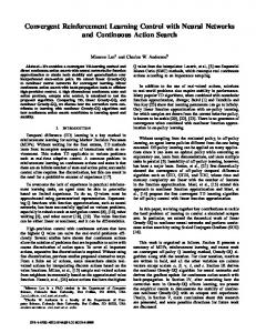
The MCRL algorithm has three parameters; α, γ and G. The learning rate is primarily controlled by α but also to some extent by G. The parameter γ regulates the discount of future rewards. The BCPNNRL System Architecture The BCPNNRL system is presented in three steps. First we present the most basic system possible with only one projection to the action-population, then we extend the system to incorporate two projections to the action-population and finally we add a value-projection and value-population to the system. The most basic BCPNNRL system was designed with two populations of units. One population was used to represent the current state of the agent, the statepopulation. The other population, the action-population, was used to represent the actions that the agent could perform. Between these two populations was a feedforward projection from the state-population to the action-population. Figure 3a shows the layout of the system used in n-armed bandit problem and Figure 3b shows the system used to solve the path finding problems in the Gridworld. Both the state- and action-population were represented with only one hypercolumn. Each unit in the state-population corresponded to a single state and each unit in the action-population corresponded to a single, elementary, action. Many biological realistic models concerned with navigation use a similar state representation [29] and this form of state representation is thought to exist in the Hippocampally place cells [24]. As mentioned earlier the activity in a single hypercolumn sum to one and in the state- and action-populations it is interpreted as a probability density functions (pdf) over the set of possible states or actions.

The BCPNNRL systems policy function was located to the action-population. The activity in the action-population was controlled by the softmax parameter G. The parameter G can solely regulate the exploitation-exploration balance and it may thus be thought of as a noradrenerigc neuromodulator [30, 31]. The parameter τP was used to regulate the learning rate. The learning rate and the balance between exploration-exploitation could in the BCPNNRL system be viewed as the same thing. Both G and τP affected the learning rate of the system and could be used to regulate it, but τP was preferably used. The parameter τE controlled the length of the eligibility trace. If τE=1 there was no trace and the system could not handle delayed rewards i.e. go through a series of states before getting the reward. If τE was increased above 1 the trace started to grove long and as the trace grove longer the learning rate became higher. If the trace was very long the gradient of the trace became very shallow which was not good for the learning. This very basic BCPNNRL system, with only one projection, could only handle positive rewards. A positive reward induced a strengthening in the connection between states and actions, in the BCPNN algorithm the strength of the print signal was determined directly by the reward. actionpopulation

state-population

action 1

state 1

action 2

state 2

actionpopulation action 1

state-population projection

projection

action 2

state 1 action3

action n-1

state n-1

action n

state n

action 4

a

b

Figure 3 Two different realisations of the most basic BCPNNRL system. In each population the active unit represents the current state and action. (a) The BCPNNRL system used in the nArmed Bandit task. The projection between the two populations contains n connections. (b) The BCPNNRL system used in the Gridworld. The feed-forward projection between the two populations contains 4n of connections.

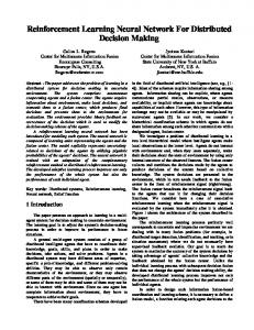
The BCPNNRL system was based on the BCPNN algorithm and each cycle or step in the agent-environment loop corresponded to a time-step in the network algorithm. Figure 4 shows the neural activity correlated to the agent-environment interaction. First the agent perceived its environment and then this information was propagated to the action-population which generated an action, a(t). After action a(t) had been performed the agent may have got a positive reward and if so the projection between the state- and action-populations was modulated in order to enhance the current and past correlations stored in the trace. The synaptic trace corresponds to the eligibility trace in regular RL algorithms. After each epoch the synaptic traces (the E-RAs) were resettled to their bias values.

An important feature of this system was that no external memory or computations were needed. All processing of information was done within the network of BCPNN units. If the BCPNN is considered to be biologically realistic then the BCPNNRL was biologically plausible structure.

a

Activate the current state

statepopulation

actionpopulation

b

Propagate the activity forward

statepopulation

actionpopulation

c

Enhance the trace of past correlations

statepopulation

actionpopulation

if r(t+1) > 0 print projection

state s(t)=2

Agent

projection

Agent

projection

action a(t)=4

reward r(t+1)=0

Agent

Figure 4 The agent-environment interaction correlated to the neural process in the BCPNN. (a) The current state is activated in the state-population, s(t)=2. (b) The activity in the statepopulation is propagated forward to the action-population and an action is generated (a(t)=4). (c) If the action a(t) in state s(t) generated a reward the projection between the state- and actionpopulations is modulated in order to enhance the past correlations stored in the trace. The reward is the input to the print signal, e.g. reward=1 generates a print signal that is 1.

The more advanced BCPNNRL system handled both positive and negative rewards and it also had the ability to relearn. The system incorporated two projections (Figure 5), one positive and one negative projection. When the system got a positive reward the positive projection was updated and the negative projection was decayed. The negative projection was update when the system got a negative reward and then the positive projection was decayed. The decay was only activated when the agent received a reward. With this extended, dual projection, BCPNNRL system came a small extension to the BCPNN algorithm; synaptic decay (eq. (15)-(17)). The synaptic decay was used to make the BCPNNRL flexible and capable of relearning. The decay meant that both of the projections were updated no matter if the print signal was positive or negative. In eq. (15)-(17) there is a variable print, which was set to the same value as the print signal. To summarize; the two projections shared the same set of parameters and the decay was as strong as the update. ∂Pi (t ) (15) = print (biasi − Pi (t )) / τ P ∂t ∂Pj (t ) (16) = print (bias j − Pj (t )) / τ P ∂t ∂Pij (t ) (17) = print (biasij − Pij (t )) / τ P ∂t

A key issue was how the input from the two projections was combined in the action-population. Here the negative projection was inverted simply by negating the support values. The result was that the input from the negated projection inhibited the units in the action-population. state-population state 1 state 2

actionpopulation pos. projection

action 1 action 2 action3

state n-1 state n

neg. projection

action 4

Figure 5 A BCPNNRL system with both a positive and negative projection to the actionpopulation. This system was capable of handling both positive and negative rewards as well as relearning. Both of the projections shared the same set of parameters and when one of the projections was updated the other one was decayed proportionally.

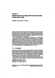
In order to not only act on reward but also act on the lack of reward we experimented with a system that had a value-population. The value-population was only activated when a reward was present and it did not form a value-function but rather a reward-function4. In appendix A different ideas of how to construct a valuefunction with the value-population are discussed. It may seem strange that the value-population had two units instead of just one. The reason is that we wanted to be able to give the system input that varied in strength and frequency and the BCPNN algorithm then required that there was at least two units in a hypercolumn. Previous BCPNNRL system presented in Figure 5 translated the reward directly into a print signal that was used to update the two action-projections. The system presented in Figure 6 computed the print signal based on the knowledge stored in the value-population, the print signal was then used to update both of the two actionprojections and the value-projection. We denote the two units in the value-population as p1 and p2. If a reward, r, was present the print signal was computed as r-p1 and then it was used to update all three projections. The activity of the two units was clamped to p1=r and p2=1-r during the update of the value-projection. It was important to note that the value-population perceived much more of positive updates (p1=1, p2=0) than of negative updates (p1=0, p2=1). This imbalance had to be corrected in order for the system to maintain its dynamics, therefore the positive updates of value-projection had only 1/50 of the strength, i.e. print signal was divided by 50, of negative updates.

4

Instead of assigning a value to each state, a reward-function only stores values in those states where an absolute reward have been received.

value-population state-population

positive

state 1

negative

value projection

state 2 state

print signal

action-population pos. projection

state n-1

action 1 action 2 action

state n

action3 neg. projection

action 4

Figure 6 A BCPNNRL system with a value-population and projection. This system could react on the lack of expected reward. The information of existence of reward was stored in the valuepopulation and this population was also used to compute the print signal when a reward was encountered. The value-population was only activated when a reward was present.

Experiments We chose to benchmark our BCPNNRL system on two tasks. The first task was the narmed bandit problem. This was considered to be a simple problem and it did not require the use of an eligibility trace. The second task was path finding in a maze and this task required the use of an eligibility trace and was considered to be medium hard. The n-Armed Bandit The n-armed bandit problem is the classical problem of selecting the action with the highest return. In the context of RL we can formulate this problem as having one state in which we can perform n different actions and the goal is to find the action that yields the highest return under the constraint that we want to maximise our total reward. The basic solution to the problem is to sample the returns from the n different actions and then chose the most beneficial. The catch is to find this optimal action in an effective way so that the total reward is maximised. In this problem taking a step, i.e. performing an action is equal to finishing an epoch. We were using both a 10- and 2-armed bandit in the experiments. In the case of the 10-armed bandit the rewards were given in a linearly increasing order from 0 to 9, e.g. action 5 yielded a reward of 4. We also evaluated the two methods in a stochastic environment where the reward 9 was given for each action but with different probabilities, e.g. action 5 yielded a reward of 9 with a probability of 0.5.

Gridworld A simple maze that we called Gridworld (Figure 7 and Figure 8) was used in many of the experiments. Each grid in the maze corresponded to a state and in each state four different actions were available; go north, east, south or west. Each performed action was a step. The task in the Gridworld was to find a reward. When the reward was found a new epoch was started and the agent was returned to its starting state. The values of the rewards were in the range of [-1,1]. The agent was allowed to make moves into a wall or into the out-of-bounds area around the maze, these moves did not affect the position of the agent but they could affect the reward.

Figure 7 A 4x4 Gridworld where the agent was starting in the lower left corner and the goal was in the upper right corner. There were four actions available to the agent; go north, east, south or west. The agent was allowed to make moves into the out-of-bound region but it did not affect the agent’s position.

Figure 8 A t-maze constructed in the Gridworld. Initially the left side gave a reward of 1 and the right side a reward of –1. After 50 epochs the positive and negative rewards switched place and this was then repeated with an interval of 50 epochs.

We mainly used the 4x4 Gridworld (Figure 7) to evaluate the BCPNNRL and MCRL methods. In order to evaluate the scaling capabilities of the methods we also used a 8x8 maze. A t-maze (Figure 8) was used to study the dynamics of the BCPNNRL system and its capabilities of relearning. In the t-maze task the left side

reward was initially 1 and the right side reward –1 or0.015. After 50 epochs the positive and negative rewards switched side, after another 50 epochs they switched side again and so fourth. The agent had to follow the positive reward as it moved from side to side in the t-maze and this could only be done by the dual projection BCPNNRL system.

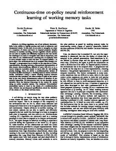
Results In the initial experiments the two methods were benchmarked, also some of the properties of the BCPNNRL system were studied. The single projection BCPNNRL system was used and the results of these initial experiments would not differ if the dual projection BCPNNRL system had been used instead since the second projection was not used. First we present the basic benchmarks, investigate the effects of different parameter settings and report on an experiment with a stochastic environment, then we move on to study the dynamics of the BCPNNRL system and the dual projection system. Finally we look at how frustration, i.e. expectation of reward, can be implemented in the BCPNNRL system. Benchmarks The first benchmark was done on the 10-armed bandit task. This benchmark, on the 10-armed bandit, showed that both of the algorithms were able to find a good solution to the problem with the given parameter setting and both of the solutions had similar characteristics (Figure 9). The reward was given immediately after each action and therefore no eligibility trace or memory of actions leading up to the reward was necessary, hence τE=1 and γ=1. The two methods were evaluated by the fraction of maximum reward they received over 100 runs e.g. if a method chose the optimal action 100 out of 100 times that gave 1. The first experiment with the Gridworld was to benchmark the two algorithms on a path-finding problem in a 4x4 maze. The goal was located in the upper right corner and the starting point was located in the lower left corner (Figure 7). This experiment was intended to characterize the solutions of the two algorithms when the reward was delayed. The measure used to evaluate the solutions was the inverse of the path length, e.g. the optimal path in the 4x4 Gridworld is 6 steps and hence a solution with 6 steps resulted in 1. Figure 10 show that both methods found a very good solution after approximately 10 epochs (Figure 10). The two methods were also benchmarked in a stochastic 10-armed bandit environment (Figure 11). We used a 10-armed bandit where the agent received a reward of 9 with different probabilities. The BCPNNRL system proved to be slightly superior to the MCRL algorithm on this task. It is also noticeable that the results were very similar to those of the deterministic 10-armed bandit.

5

The reward 0.01 and not 0 is given because it simplifies the implementation of the algorithm; it has no effect on the BCPNNRL system which of these two values is used.

1

BCPNNRL

Fraction of Maximum Reward

0.9 0.8 0.7

MCRL

0.6 0.5 0.4 0.3 0.2 0.1 0

50

100

150

200

250

300

350

400

Epochs

Figure 9 The MCRL algorithm and BCPNNRL system solved the 10-armed bandit problem. The 10 arms (actions) gave a reward ranging from 0 to 9 and the task was to find the arm that returned the highest reward. The results were averaged over 100 runs. MCRL parameters: γ=1, α=0.02, G=1 BCPNNRL parameters: τE=1, τP=100, G=1 1

Inverse of Optimal Solution

0.9 0.8

MCRL

0.7

BCPNNRL 0.6 0.5 0.4 0.3 0.2 0.1 0

5

10

15

20

25

30

Epochs

Figure 10 The path-finding problem in a 4x4 maze. This task required that the agents could handle delayed rewards. The result was averaged over 100 runs. MCRL parameters: γ=0.99, α=0.3, G=60 BCPNNRL parameters: τE=2, τP=5, G=3

1

Fraction of Maximum Reward

0.9

BCPNNRL

0.8 0.7

MCRL

0.6 0.5 0.4 0.3 0.2 0.1 0

50

100

150

200

250

300

350

400

Epochs

Figure 11 The two methods were benchmarked in a stochastic 10-armed bandit environment. The reward was constantly 9 but the chance of getting the reward varied between the actions. Choosing action a9 returned a reward 90% of the times, choosing action a8 gave a reward 80% of the times and so forth. Finally choosing action a0 never returned any reward. The result was averaged over 100 runs. MCRL parameters: γ=1, α=0.02, G=1 BCPNNRL parameters: τE=1, τP=100, G=1

Learning Rate In order to illustrate how the learning rate of the BCPNNRL was affected by different parameter settings we did four experiments, using the 10-armed bandit, with different parameter settings (Figure 12). The learning rate of the BCPNNRL system was controlled by the parameters G and τP. In the upper plot, G was small and the learning rate was low, in the lower plot G was large and the learning rate was high. In both the lower and upper plot the effect of τP was obvious, a small value of τP meant a high learning rate and vice versa. This means that an increased value of G has the same effect as a decreased value of τP – the learning rate goes up and vice versa. As mentioned previously if the learning rate is very high the agent risks not finding the optimal solution but on the other hand a slow learning rate is not good in a shortterm perspective.

Fraction of Maximum Reward Fraction of Maximum Reward

1 0.8 0.6

τP=30 τP=100

0.4 0.2 0

1

50

100

150

200 Epochs

250

300

350

400

150

200 Epochs

250

300

350

400

τP=500

0.8 0.6

τP=1500

0.4 0.2 0

50

100

Figure 12 The two plots illustrate how the parameters G and τP affected the learning rate in the 10-armed bandit task. In the upper plot the value of G was small and in the lower plot the value was large. In both the upper and lower plots two different values of τP was used, one small and one large value. The effect of a large G value was that the learning rate was high, but the effect of a large τP was that the learning rate was low. These two parameters, G and τP, had a very similar effect on the BCPNNRL system. The result was averaged over 100 runs. Upper plot BCPNNRL parameters: τE=1, G=1; Lower plot BCPNNRL parameters: τE=1, G=5

Trace Length To illustrate the effect of the trace length, the E variable, we ran the BCPNNRL system with two different trace lengths (values of τE). One version of the BCPNNRL had a short trace (τE=2) and the other had a long trace (τE=4). In the small 4x4 Gridworld the solution was not significantly affected by the trace-length (upper plot, Figure 13). But in the larger 8x8 Gridworld the solution of the BCPNNRL with the short trace was really hampered by the trace’s rapid decay (lower plot, Figure 13). The results in Figure 13 shows that the length of the trace limits the size of the problem that the BCPNNRL system can solve. If the trace is made longer the BCPNNRL system can solve larger problems, but the quality of the solutions then gets poor. A long trace is very flat and it contains less information about the direction to the goal than a short trace. It is important to point out that when the trace is made longer i.e. the value of τE is increased the trace also gets shallower which means that the signal-to-noise ratio for the trace goes down. To compensate for the shallower trace and still attain a stable solution the G parameter must be increased.

Inverse of Optimal Solution Inverse of Optimal Solution

1 0.8

τE=4 τE=2

0.6 0.4 0.2 0

50

100

150 Epochs

200

250

300

200

250

300

1 0.8

τE=4

0.6

τE=2

0.4 0.2 0

50

100

150 Epochs

Figure 13 Two different lengths of the trace was used when solving the path-finding problem. The upper plot shows the results from a 4x4 Gridworld and the lower plot shows the results from a 8x8 Gridworld. The results were averaged over 100 runs. BCPNNRL parameters: τP=40, G=3

Two Projections to the Action-Population In the following experiments we were using the more advanced BCPNNRL system with two projections to the action-population. The dual projection system allowed the agent not only to learn what actions were good but also what actions were poor or even harmful. The benefit from a second projection is illustrated with an experiment in a 4x4 Gridworld where a negative reward of -1 was imposed on all moves that lead into a wall. Figure 14 shows a comparison between a BCPNNRL agent that only gets a positive reward when it reaches the goal and one agent that also gets the negative rewards when it hits the walls. The agent that also got negative rewards learned faster in the beginning because it quickly learnt what moves to avoid. The most important aspect of the dual projection BCPNNRL system is that it is capable of dynamical relearning which enables an agent to coup with a non-stationary environment. The dynamical capabilities of the dual projection system were evaluated in a tmaze showed in Figure 5. A reward was placed both in the right (reward=+1) and left (reward=-1) arm of the t-maze. After 50 epochs the rewards shifted place so that the right armed contained a negative reward and the left arm had the positive reward. The rewards then alternated forth and back during 300 epochs. Figure 15 shows the result from the experiment, the upper plot shows the learning curve for the goal in the left arm and the lower plot shows the learning curve for the goal in the right arm.

1


0.9

both pos. & neg. rewards

0.8 0.7

no neg. rewards

0.6 0.5 0.4 0.3 0.2 0.1 0

5

10

15

20

25

30

35

40

Epochs



Figure 14 Comparison of an agent that only got a positive reward when it reached the goal and one that also got negative rewards when it hit the walls. The result was averaged over 100 runs. BCPNNRL parameters: τE=2, τP=15, G=3

1 LEFT GOAL 0.8 0.6 0.4 0.2 0

0

50

100

150 Epochs

200

250

300

1 RIGHT GOAL

0.8 0.6 0.4 0.2 0

0

50

100

150 Epochs

200

250

300

Figure 15 The agent alternated between two goals. First the agent went to the left in the t−maze where the positive reward was located and the corresponding (upper plot) learning curve went up. When the positive reward was relocated to the right arm of the t-maze the agent unlearned the old path and then relearned to go right (lower plot). Between each switch 50 epochs were accomplished. The result was averaged over 100 runs. BCPNNRL parameters: τE=2, τP=5, G=3

An important question was if it was possible to get an agent, based on the BCPNNRL system, to choose an action with a certain frequency. The answer was yes, if the dual

projection BCPNNRL system was used and no if the single projection system was used. The experiment in Figure 16 was made on a 2-armed bandit and two approaches were taken, one deterministic and one stochastic. In the experiment the agent could chose between two actions, UP and DOWN. The agent’s task was to select the UP action 70% and the DOWN action 30% of the times? The deterministic approach with a single projection gave the reward 0.7 when the UP-action was selected and 0.3 when the DOWN-action was selected (Figure 16, upper plot – one projection). When the dual projection system was used and the UPaction selected, a reward of 0.7 was given to the positive projection and 0.3 was given to the negative projection and vice versa when the DOWN-action was selected (Figure 16, upper plot – two projections). The stochastic approach was to give the reward 1 with a probability of 70% if the UP-action was selected and if the DOWN-action was selected a reward of 1 was given with a probability of 30% (Figure 16, lower plot – one projection). The dual projection system gave the reward 1 with a probability of 70% and –1 with a probability of 30% if the UP-action was selected. If the DOWN-action was selected a reward of 1 was given with a probability of 30% and –1 was given with a 70% probability (Figure 16, lower plot – two projections). Fraction of UP-action

1 One projection 0.8 0.6

Two projections

0.4 0.2 0

50

100

150

200 Epochs

250

300

350

400

250

300

350

400

Fraction of UP-action

1 One projection 0.8 0.6

Two projections

0.4 0.2 0

50

100

150

200 Epochs

Figure 16 The task was to select the UP-action 70% of the times in a 2-armed bandit. A running average was computed over the actions selected by the agents. Two different approaches were considered, one deterministic (upper plot) and one stochastic (lower plot). A BCPNNRL system with one projection could not maintain a constant level of exploration instead it saturated in both the deterministic and stochastic case to selecting the UP-action. The results were averaged over 500 runs. BCPNNRL parameters: τE=1, τP=15, G=1

The system with only one projection was not able to achieve a constant level of exploration instead it saturated to only select the UP-action. The dual projection

system chose the UP-action with the correct frequency because the two projections managed to balance each other. Estimating Reward This experiment was intended to show that a BCPNNRL system with a valuepopulation could react not only on reward but also on the lack of reward. We compared the results of the BCPNNRL system with those of the MCRL algorithm.


1 LEFT GOAL 0.5 0

0

50

100

150

200

250

300

1 RIGHT GOAL 0.5 0

0

50

100

150

200

250

300


1 LEFT GOAL 0.5 0

0

50

100

150

200

250

300

1 RIGHT GOAL 0.5 0

0

50

100

150 Epochs

200

250

300

Figure 17 A dual projection BCPNNRL system with a value-population performed the t-maze task with shifting rewards. The upper two plots shows the result when the reward shifted between 1,-1. The lower two plots shows the result when the reward shifted from 1 to 0.01. The print signal for the positive value-projection was scaled down with a factor of 0.02. The results were averaged over 100 runs. BCPNNRL parameters; value prj.: τE=1, τP=10, G=1, action prj.: τE=2, τP=2, G=3.

The experiment was performed in the t-maze where a reward was placed both in the right and left arm as described in previous section. The two upper plots in Figure 17 and Figure 18 were made when the rewards shifted between 1 and –1. The two lower plots in Figure 17 and Figure 18 were made when the rewards alternated between 1 and 0.01. As previously the rewards shifted side after 50 epochs and this process continued for 300 epochs. Although a reward of 0.01 was not negative, if this small reward was given after a period of larger positive rewards the system interpreted it as a punishment i.e. a negative reward (Figure 17, lower plots).


It proved hard to balance the positive and negative updates of the value-projection since the agent always tried to maximise its positive updates and therefore avoided the negative updates. This was especially critical when we wanted the BCPNNRL system to react on the lack of reward, i.e. when the rewards alternated between 1 and 0.01. A factor of 0.02 was used to scale to the print signal to the positive updates of the valueprojection. The balance problem could also somewhat be remedied by imposing negative rewards on those actions that led into the walls. The MCRL algorithm was able to perform well on the t-maze task when the rewards shifted between 1 and 0.01, but when the rewards alternated between 1 and – 1 it failed to find a good solution. When the rewards were 1 and –1 the MCRL algorithm quickly learnt that neither of the two arms were good and therefore it did nothing, except running into to the walls. It did not help if a negative reward was put on the moves that led into the walls. 1 LEFT GOAL 0.5 0 1

50

100

150

200

250

300

RIGHT GOAL 0.5 0


0

1

0

50

100

150

200

250

300

LEFT GOAL 0.5 0 1

0

50

100

150

200

250

300

RIGHT GOAL 0.5 0

0

50

100

150 Epochs

200

250

300

Figure 18 The MCRL algorithm performing the same task as the BCPNNRL system in Figure 17. The result was averaged over 100 runs. MCRL parameters: γ=0.99, α=0.3, G=60

Discussion The experiments show that the BCPNNRL is able to match the performance of the standard MCRL algorithm. Both of the two methods have the same number of parameters and use similar policy functions. The two implementations base their knowledge on sample returns and they are both on-policy methods. The BCPNNRL algorithm showed to be very versatile and it could easily cope with a stochastic environment. The BCPNNRL algorithm is based on the BCPNN and since the BCPNN is derived from statistical considerations it is only natural that the BCPNNRL handles the stochastic environment well. We did not experiment with stochastic state representations or partially observable states, i.e. two separate states that looks the same to the agent. It would also be interesting to study the BCPNNRL capabilities on a partially observable Markov decision process or POMDP and compare its performance to learning rules based on hidden Markov models or HMM. The built in policy function of the BCPNNRL, based on the Gibbs distribution, proved to be good. The BCPNNRL based agent seeks out the optimal path and the policy aids it to avoid the worst moves and direct the exploration of the state-space. We can also conclude that there is a close relationship between the learning rate and the policy, by regulating the learning rate you implicitly regulate the policy. If the parameters of the BCPNNRL system are matched to those of the MCRL algorithm it is easy to understand that the gain, G, have the same effect in both of the two methods i.e. regulating the policy. The parameter τP in the BCPNNRL system corresponds to α in the MCRL algorithm, these two parameters regulate the learning rate. Setting α=1 corresponds to having τP=1 and increasing τP corresponds to decreasing α. The connection between τE and γ is not obvious but both of these two parameters are used to regulate the degree of discount put on future rewards. Letting τE→∞ corresponds to letting γ→1. The BCPNNRL parameters τP and G are somewhat dependent i.e. they have a similar effect on the solution just as the MCRL parameters α and G. The parameter τE can in some cases, where the path length is within the scope of the trace length, be thought of as a constant and the same is true for the MCRL parameter γ. The BCPNNRL system with two projections to the action-population and no valuepopulation is insensitive to noise and parameter settings. The dual projection system proved to be able to balance its exploration rate and perform well in a non-stationary environment. When a value-population is added to the system it becomes more sensitive to parameter settings but the system also becomes more powerful. With the valuepopulation the BCPNNRL system can react on the lack of reward, i.e. be frustrated. Representing a reward-function with a separate value-population that is not dependent on the action-population may not be a good thing to do. Especially not if one want to construct some form TD-learning system. But separating out the valuefunction allows a more biologically plausible system since no complicated external calculations are needed. Evaluating the performance of the t-maze problem is not straight forward, the MCRL algorithm fails to find a solution when the rewards are shifted between 1 and

–1. This may not be a bad thing since apparently both of the goals on either side of the t-maze punish the agent from time to time. The BCPNNRL system is, as all types of sample return based RL systems, best suited for small problems. When the problem is large it is very advantageous to use RL methods that are based on TD-learning. An important aspect of the BCPNNRL system is that it can be fully implemented with a BCPNN. No “external” short-term memory is needed and the backup performed in the MCRL algorithm comes as an intrinsic part of the BCPNN units. This means that if the BCPNN is considered to be a biologically plausible model then the BCPNNRL is a biologically plausible system. Instead of using only one hypercolumn it is possible to have several hypercolumns in either the state- or action-population. The coding then becomes distributed and this can increase the noise tolerance in a noisy system. Distributed coding also simplifies the pre-processing of input data (used to represent the states) since the input can be mapped directly from the sensors into the BCPNN and the BCPNNRL system. The populations can have one or several feedback or recurrent projections. This means that e.g. the states may be represented as attractor memories. It is also a conceivable idea to have high order action hierarchies instead of only elementary actions. A continuous time implementation of the BCPNN algorithm was not used in the BCPNNRL system. In a future implementation it would be interesting to make a stronger connection, use an absolute time, between the time in the agent-environment and the BCPNN algorithm. In further studies it would be interesting to investigate how temporal difference (TD) rewards can be incorporated into the BCPNNRL system. The advantages of TDlearning are many and a system that uses it has the ability to predict future rewards and react when these rewards are no longer present. A TD approach also reduces the importance of the trace-length and would allow a BCPNNRL based system to find solutions of any size. The current version of the BCPNNRL system is primarily focused on locating a single goal i.e. pursuing a single desire. In a real world application an agent probably has to be able to pursue several goals or desires i.e. locate both food and water. Such a system could be constructed by combining several units of the basic BCPNNRL system. The new, larger, system would have a structure similar to that of the BCPNNRL system with the difference that the state-space is replaced by the output from all of the BCPNNRL systems. A difficult problem to solve in the new system is how to balance the decision making between the BCPNNRL systems constituting it.

Appendix A, Temporal-Difference Learning and BCPNN A central part of TD-learning is to construct a value-function i.e. assigning each state a value based on its relative position to the reward or goal. Here we present two ways of constructing a value-function and both of these methods are based on the system with a value-population (Figure 6). The first approach uses delayed rewards (E-traces) and the second approach uses future rewards (Z-traces). Unfortunately neither of these attempts to construct a BCPNNRL system capable of TD-learning proved successful. A complication that exists in both of these attempts is that the action-values and state-values are separated and updated independently. Therefore the GPI cycle is not followed as intended. Temporal Difference Learning with E-trace This approach was derived from the reward prediction system. The idea was simply to add a synaptic trace or E-trace to the value-projection identical to that of the actionprojection. This meant that each state was assigned its own particular value instead of only letting the end-state, where the reward was located, to have a value. In each state we wrote; p1=1 and p2=0, where the two units p1 and p2 were located in the value-population. The print signal was computed by comparing the values of the p1 unit between two consecutive states. The experiments performed with this model did not give truly positive results. The system was able to find a single goal in the Gridworld but it was not able to coup with alternating rewards in the t-maze, especially not when the rewards 1 and 0.01 were used. Temporal Difference Learning with Z-trace We investigated the possibility of adding a Z-trace, which would enable the construction of a value-function. The Z-trace is formulated in eq. (18) and (19) where the variables Zi and Zj are intended to replace Si and Sj in eq. (1)-(3). These two new equations represents the synaptic potential in the pre- and postsynaptic synapses and the parameters τZpre and τZpost are in the range of [1,∞). ∂Z i (t ) (18) = ( Si (t ) − Z i (t )) / τ Zpre ∂t ∂Z j (t ) (19) = ( S j (t ) − Z j (t )) / τ Zpost ∂t In each state the values of the two units p1 and p2 in the value-population was read and printed (printed in the same state as they were read). The print-signal was, as earlier described, computed by comparing the values of the p1 unit between two consecutive states. The Z-trace propagated the value of the two p units backwards to the previous state’s p unit-values. The resulting system proved to be able to find a single goal in the Gridworld but it did not manage to follow the alternating positive reward in the t-maze. A possible reason to the failure of this approach maybe that the GPI paradigm is violated.

References 1. 2. 3. 4. 5. 6. 7. 8. 9. 10. 11. 12.

13. 14. 15.

16. 17. 18. 19. 20.

21. 22.

23.

Mitchell, T., Machine Learning. 1997: McGrawHill. Rusell, S. and P. Norvig, Artificial Intelligence: A Modern Approach. 1995: Prentice Hall. Kaelbling, L.P., M.L. Littman, and A.W. Moore, Reinforcement Learning: A Survey. Journal of Artificial Intelligence Research, 1996. 4: p. 237-285. Sutton, R.S. and A.G. Barto, Reinforcement Learning: An Introduction. 1998: MIT Press. Hertz, J., A. Krogh, and R.G. Palmer, Introduction to the Theory of Neural Computation. 1991: Addison-Wesely. Haykin, S., Neural Networks: A Comprehensive Foundation. 2 ed. 1999: Prentice Hall. Schraudolph, N.N., P. Dayan, and T.J. Sejnowski. Temporal Difference Learning of Position Evaluation in the Game of Go. in NIPS 6. 1994. San Francisco. Thrun, S. Learning to Play the Game of Chess. in NIPS 7. 1995. Tesauro, G., Temporal difference learning and TD-Gammon. Communications of the ACM, 1995. 38(3): p. 58-68. Sporns, O. and W.H. Alexander, Neuromodulation and plasticity in an autonomous robot. Neural Networks, 2002. 15(4-6): p. 761-774. Gadanho, S.C. and J. Hallam, Robot Learning Driven by Emotions. Adaptive Behavior, 2001. 9(1): p. 42-64. Barto, A.G., R.S. Sutton, and C.W. Anderson, Neuronlike adaptive elements that can solve difficult learning control problems. IEEE Transactions on Systems, Man and Cybernetics, 1983. SMC-13: p. 834-846. Dayan, P. and T.J. Sejnowski, Exploration Bonuses and Dual Control. Machine Learning, 1996. 25: p. 5-22. McCulloch, W.S. and W. Pitts, "A logical calculus of the ideas immanent in nervous activity". Bulletin of Mathematical Biophysics, 1943. 5: p. 115-133. Hopfield, J.J., Neural networks and physical systems with emergent collective computational abilities. Proceedings of the National Academy of Sciences, 1982. 79: p. 2554-2558. Kohonen, T., Self-organized formation of topologically correct feature maps. Biological Cybernetics, 1982. 43: p. 59-69. Rumelhart, D.E., G.E. Hinton, and R.J. Williams, Learning representations by backpropageting errors. Nature, 1986. 323: p. 533-536. Lansner, A. and Ö. Ekeberg, A one-layer feedback artificial neural network with a Bayesian learning rule. Int. J. Neural Systems, 1989. 1: p. 77-87. Sandberg, A., et al., A Bayesian attractor network with incremental learning. Network: Computation in Neural Systems, 2002. 13(2): p. 179-194. Holst, A. and A. Lansner, A Higher Order Bayesian Neural Network for Classification and Diagnosis, in Applied Decision Technologies: Computational Learning and Probabilistic Reasoning, A. Gammerman, Editor. 1996, John Wiley & Sons Ltd.: New York. p. 251-260. Johansson, C., A. Sandberg, and A. Lansner. A Neural Network with Hypercolumns. in ICANN. 2002. Spain, Madrid: Springer-Verlag Berlin. Hubel, D.H. and T.N. Wiesel, Uniformity of monkey striate cortex: A parallel relationship between field size, scatter and magnification factor. J. Comp. Neurol., 1974(158): p. 295-306. Hebb, D.O., The Organization of Behavior. 1949, New York: John Wiley Inc.

24.

25. 26. 27. 28.

29.

30. 31.

Kandel, E.R., J.H. Schwartz, and T.M. Jessell, The Anatomical Organization of the CNS, Coding of Sensory Information, in Principles of Neural Science. 2000, McGraw-Hill Companies. p. 318-336, 411-429. Marder, E. and V. Thirumalai, Cellular, synaptic and network effects of neuromodulation. Neural Networks, 2002. 15(4-6): p. 479-493. Reynolds, J.N.J. and J.R. Wickens, Dopamine-dependent plasticity of corticostriatal synapses. Neural Networks, 2002. 15(4-6): p. 507-521. Deneve, S., P.E. Latham, and A. Pouget, Reading population codes: a neural implementation of ideal observers. Nature, 1999. 2(8): p. 740-745. Carandini, M., D.J. Heeger, and J.A. Movshon, Linearity and Normalization in Simple Cells of the Macaque Primary Visual Cortex. The Journal of Neuroscience, 1997. 17(21): p. 8621-8644. Foster, D.J., R.G.M. Morris, and P. Dayan, Models of Hippocampally Dependent Navigation, Using The Temporal Difference Learning Rule. Hippocampus, 2000. 10: p. 1-16. Usher, M., et al., The Role of Locus Coeruleus in the Regulation of Cognitive Performance. Science, 1999. 283: p. 549-554. Doya, K., Metalearning and neuromodulation. Neural Networks, 2002. 15(4-6): p. 495-506.