Convergent Reinforcement Learning Control with Neural Networks and Continuous Action Search Minwoo Lee1 and Charles W. Anderson2 Abstract—We combine a convergent TD-learning method and direct continuous action search with neural networks for function approximation to obtain both stability and generalization over inexperienced state-action pairs. We extend linear Greedy-GQ to nonlinear neural networks for convergent learning. Direct continuous action search with back-propagation leads to efficient high-precision control. A high dimensional continuous state and action problem, octopus arm control, is examined to test the proposed algorithm. Comparing TD, linear Greedy-GQ, and nonlinear Greedy-GQ, we discuss how the correction term contributes to learning with nonlinear Greedy-GQ algorithm and how continuous action search contributes to learning speed and stability.
I.
I NTRODUCTION
Temporal difference (TD) learning is a key method in reinforcement learning for solving Markov Decision Processes (MDPs). Without waiting for the final returns, TD methods learn from incomplete sequences of interactions with an environment. This makes TD applicable to various problems such as real-time adaptive control. A common problem in reinforcement learning on continuous actions and states is that there are an infinite number of state and action pairs; successful control often requires fine discretization, but this can result in the need for a prohibitive amount of experience [17]. To overcome the lack of experience in practical reinforcement learning tasks, an agent must be able to generalize based on limited experience. To do so, Q-values must be approximated using parameterized representation. Representing Q functions with function approximations, such as neural networks, has been successfully applied on various problems, especially in robotics such as navigation control [6], [10], robot walking [2], and robot soccer [18], [19]. The value function can be either linear or nonlinear, and it can be differentiable. High-precision control with continuous actions that have the highest Q value can solve the real-world problems efficiently. Several studies have shown that continuous actions allow the solution of problems that are impossible to solve with coarse discretization of action space. To cover all important actions, expensive fine discretization is required. Without using fine discretization, previous studies proposed alternative ways. From a finite set of actions, some researchers obtain realvalued actions by interpolating discrete actions based on the value functions. Millan, et al., [15] sample real-valued actions from neighbors incrementally based on the approximated value function. Hasselt, et al., [24] select actions that have the highest 1 Minwoo Lee is a Ph.D student in the Department of Computer Science, Colorado State University, Fort Collins, CO 80523, USA
[email protected]
2 Charles W. Anderson is a faculty of the Department of Computer Science, Colorado State University, Fort Collins, CO 80523, USA
[email protected]
978-1-4799-4552-8/14/$31.00 ©2014 IEEE
Q value from the interpolator. Lazaric, et al., [3] use Sequential Monte Carlo (SMC) methods, which resample real continuous actions according to an importance sampling. In addition to the use of real-valued actions, solutions to real-world problems also require stability in performance. Many popular TD algorithms, when combined with nontabular function approximation, diverge; Baird [1] and Tsitsiklis and Van Roy [23] show that learning parameters can go to infinity. Only linear function approximation with on-policy learning, for which samples are drawn from the current behavior policy, is known to be stable [20], [22], [23]. There is no guarantee of convergence when combined with nonlinear function approximation in on-policy learning. Without sampling from the evaluated policy, in off-policy learning, an agent learns policies different from the one being executed. Off-policy learning can be applied on many applications since it can learn an optimal policy while executing an exploratory one, learn from demonstrations, and learn multiple tasks in parallel [5]. Instability of off-policy learning, however, has been a major issue. Sutton, et al., [21] first theoretically showed the convergence of off-policy temporal difference algorithm such as GTD, GTD2, and TDC, whose time and memory complexity are linear with the number of features in the function approximation. Maei, et al., [13] extend this approach to nonlinear function approximation and Maei, et al., [14] propose the first convergent TD learning algorithm for off-policy control with linear function approximation. In this paper, we bring together key contributions to tackle the hard problem of learning to control a simulated octopus arm. In particular, we extend the theoretical work of linear Greedy-GQ to nonlinear neural networks and perform continuous action search by using Scaled Conjugate Gradient (SCG) [16]. This work is organized as follows. Section II presents a summary of MDPs, reinforcement learning, and recent work on convergent off-policy Q learning method, Greedy-GQ algorithm along with the notation. For clear notation, matrices are written in bold, and all the other variables are column vectors except scalars 𝛼, 𝛽, 𝛾, 𝛿, and 𝜖. Section III derives the nonlinear Greedy-GQ algorithm for neural networks and derives the gradient update for continuous action search with back-propagation. In Section IV, after examining how the correction term in Greedy-GQ affects learning, we present the empirical results to demonstrate the stability of continuous nonlinear Greedy-GQ with an octopus arm experiment. Finally, in Section V, main conclusions about this research are presented, and some possible directions for future work are discussed.
II.
T EMPORAL D IFFERENCE L EARNING AND G REEDY-GQ
As developed in dynamic programming and Monte Carlo methods, Temporal difference (TD) learning uses bootstrapping to update the value estimates. A Markov decision process 𝑎 (MDP) is defined as a tuple (𝑆, 𝐴, 𝑃𝑠𝑠 ′ , 𝑅, 𝛾), where for each 𝑎 time step 𝑡 = 0, 1, 2, ⋅ ⋅ ⋅ , with probability 𝑃𝑠𝑠 ′ , action 𝑎𝑡 ∈ 𝐴 in state 𝑠𝑡 ∈ 𝑆 transitions to state 𝑠𝑡+1 = 𝑠′ ∈ 𝑆, and the environment emits a reward 𝑟𝑡+1 ∈ 𝑅. The value function 𝑉 𝜋 for a policy 𝜋 : 𝑆 → 𝐴 is defined as: 𝜋
𝑉 (𝑠) = 𝔼[
∞ ∑
𝑡
𝛾 𝑟𝑡+1 ∣𝑠𝑡 = 𝑠, 𝜋],
𝑡=0
where 𝛾 is a discounting factor. The value function satisfies the following Bellman equation: 𝑉 𝜋 (𝑠) = 𝑇 𝜋 𝑉 𝜋 (𝑠) = 𝑅𝜋 (𝑠) + 𝛾𝑃 𝜋 𝑉 𝜋 (𝑠), where 𝑅𝜋 (𝑠) is a reward function for the state 𝑠, 𝑃 𝜋 is the state transition probability under the policy 𝜋, and 𝑇 𝜋 is known as a Bellman operator. Similarly, for control problems, we can define the action value method, 𝑄𝜋 (𝑠, 𝑎): 𝜋
𝑄 (𝑠, 𝑎) = 𝔼[
∞ ∑
𝑡
𝛾 𝑟𝑡+1 ∣𝑠𝑡 = 𝑠, 𝑎𝑡 = 𝑎, 𝜋].
𝑡=0
When a value function approximation 𝑄𝜃 is linear, it is defined as 𝑄𝜃 (𝑠, 𝑎) = 𝜙(𝑠, 𝑎)⊤ 𝜃, where 𝜙 is a feature vector for state 𝑠 and action 𝑎, and 𝜃 ∈ ℝ𝑑 is a 𝑑 dimensional weight vector. Action 𝑎 can be selected either greedily or randomly. To balance the limited experience from greedy action selection and suboptimal random action selection, an action can be chosen greedily most of the time but randomly with small probability 𝜖—this is called 𝜖-greedy. Off-policy TD control known as Q-learning directly approximates 𝑄∗ = max𝑎 𝑄(𝑠, 𝑎), the optimal actionvalue function, which is independent of the policy being followed. Thus, the temporal difference error in Q-learning is defined as 𝛿𝑡 = 𝑟𝑡+1 + 𝛾 max𝑎 𝑄(𝑠𝑡+1 , 𝑎) − 𝑄(𝑠𝑡 , 𝑎𝑡 ), and the algorithm has the update rule 𝜃𝑡+1 = 𝜃𝑡 + 𝛼𝑡 𝛿𝑡 𝜙𝑡 , where 𝛼𝑡 is a learning rate, and 𝜙𝑡 = 𝜙(𝑠𝑡 , 𝑎𝑡 ). Although TD is known to converge for on-policy control, there is no guarantee in off-policy problems [9]. Greedy-GQ [12], [14] is proved convergent in the mean square projected Bellman error (MSPBE) using stochastic gradient descent. To simplify the notation, removing 𝜋 and omitting the arguments for 𝑄, another objective function, MSPBE 𝐽(𝜃), can be written as: J(𝜃) = ∥𝑄𝜃 (𝑠, 𝑎) − Π𝑇 𝑄𝜃 (𝑠, 𝑎)∥2𝜇
= 𝔼[𝛿(𝜃)∇Q⊤ ]⊤ 𝔼[∇Q∇Q⊤ ]−1 𝔼[𝛿(𝜃)∇Q],
where the projection operator Π = 𝜙(𝜙⊤ 𝐷𝜙)−1 𝜙⊤ 𝐷, and 𝐷 is a diagonal matrix whose diagonal values are the probability distribution ∫ 𝜇(𝑠, 𝑎) over the state-action pairs. The norm ∥𝑄∥2𝜇 = 𝑄2 (𝑠, 𝑎)𝜇(𝑑𝑠, 𝑑𝑎). We denote the gradient of Q w.r.t. 𝜃 at 𝑠 and 𝑎 by ∇Q. Including the inverse matrix, 𝑔 ∗ can be defined from J(𝜃): ∗
⊤ −1
𝑔 = 𝔼[∇Q∇Q ]
𝔼[𝛿(𝜃)∇Q].
To avoid computation of the inverse matrix, Greedy-GQ estimates 𝑔 ∗ by 𝑔𝑡 along with the weight vector 𝜃𝑡 . Now, from
MSPBE, the gradient descent learning Greedy-GQ updates weights as follows: 𝜃𝑡+1 = 𝜃𝑡 + 𝛼𝑡 𝛿𝑡 𝜙𝑡 − 𝛼𝛾𝜙′𝑡 (𝜙⊤ 𝑡 𝑔𝑡 ),
𝑔𝑡+1 = 𝑔𝑡 + 𝛽𝑡 (𝛿𝑡 − 𝜙⊤ 𝑡 𝑔𝑡 )𝜙𝑡 ,
where 𝜙′𝑡 = 𝜙(𝑠′ , 𝑎′ ) and 𝛽𝑡 > 𝛼𝑡 . The term −𝛼𝛾𝜙′𝑡 (𝜙⊤ 𝑡 𝑔𝑡 ) is a correction term for the gradient descent direction. III.
F UNCTION A PPROXIMATION WITH N EURAL N ETWORKS
To overcome the curse of dimensionality that arises with tabular function approximation, several approaches such as neural networks, radial basis functions, fuzzy sets, and support vector machines have been proposed. Neural networks is widely used as function approximators to represent nonlinear Q function. The following derivation leads to nonlinear GreedyGQ algorithm with neural networks. A. Nonlinear Greedy-GQ Similar to the extension of linear TDC [21] to nonlinear TDC [13], we can extend linear Greedy-GQ [14] to nonlinear Greedy-GQ as follows: ) ( 𝜃𝑡+1 = Γ 𝜃𝑡 + 𝛼𝑡 𝛿𝑡 𝜙𝑡 − 𝛼𝛾𝜙′ (𝜙⊤ 𝑡 𝑔 𝑡 ) − 𝛼 𝑡 ℎ𝑡 , 𝑔𝑡+1 = 𝑔𝑡 + 𝛽𝑡 (𝛿𝑡 − 𝜙⊤ 𝑡 𝑔𝑡 )𝜙𝑡 ,
2 ℎ𝑡 = (𝛿𝑡 − 𝜙⊤ 𝑡 𝑔𝑡 )∇ 𝑄𝜃𝑡 (𝑠𝑡 )𝑔𝑡 .
where 𝜙𝑡 = ∇𝜃 𝑄(𝑠𝑡 , 𝑎𝑡 ), and Γ : ℝ𝑑 → ℝ𝑑 is a mapping that projects the weights onto a smooth boundary parameter space. The projection mapping prevents the parameters from diverging in the early stage of the algorithm because of nonlinearities. A particular definition of Γ is used to prove convergence [12], but in practice, Γ(𝑥) = 𝑥 is often used and is used here as well. B. Greedy-GQ(0) with Neural Networks Function approximation for 𝑄v,𝑤 (𝑠, 𝑎) is computed by two-layer neural networks where v is the weight matrix for the hidden layer and 𝑤 is the weight vector for the output layer. The forward pass for Q can be defined as: 𝑧 = ℎ(𝑥⊤ v) 𝑧𝑚 = ℎ(𝑥⊤ 𝑣 (𝑚) ) 𝑦 = 𝑄v,𝑤 (𝑠, 𝑎) = 𝑧𝑤 = ℎ(𝑥⊤ v)𝑤 When ℎ = tanh is the activation function, ∇ℎ = (1 − ℎ2 ), so we have the following gradient of 𝑄 w.r.t. the weight vector 𝑣 (𝑚) for hidden unit 𝑚: 𝜙𝑣(𝑚) = ∇𝑣(𝑚) 𝑄(𝑠, 𝑎) = 𝑤𝑚 ∇𝑣(𝑚) (ℎ(𝑥⊤ 𝑣 (𝑚) )) = 𝑤𝑚 (1 − 𝑧𝑚 2 )𝑥⊤
The 𝜙v can be denoted as the following matrix, and from this, we can rewrite the vector 𝜙𝑣(𝑚) as a 𝑚-th row of 𝜙v matrix. 𝜙v = ∇𝑣 𝑄(𝑠, 𝑎) = 𝑤 ⊙ (1 − 𝑧 2 )⊤ 𝑥⊤ 𝜙𝑣(𝑚) = [𝜙v ]𝑚 ,
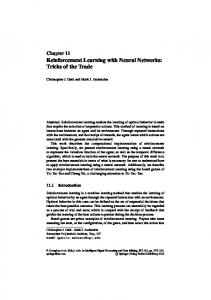
Algorithm 1 Nonlinear Greedy-GQ(0) with 2-layer neural networks Initialization: 𝑔0 to 0, v0 and 𝑤0 as random values. Choose proper small positive learning rate 𝛼v , 𝛼𝑤 , 𝛽v and 𝛽𝑤 , and set values for 𝛾 ∈ (0, 1]. Repeat for each episode: Select 𝑎 from 𝑠 by ActionSelection() to arrive at 𝑠𝑡+1 . ∗ Observe sample, (𝑠, 𝑎, 𝑟, 𝑠′ ) at time step 𝑡, where 𝑞 ′ = ′ ′∗ ′∗ ′ 𝑄v,𝑤 (𝑠 , 𝑎 ), 𝑎 = argmax𝑎 𝑄v,𝑤 (𝑠 , 𝑎). for each observed sample and 𝑄v,𝑤 (𝑠, 𝑎) = 𝑤⊤ 𝑧 where 𝑥 = 𝑥(𝑠, 𝑎), 𝑥′ = 𝑥(𝑠′ , 𝑎′ ), 𝑧 = tanh(𝑥⊤ v), and 𝑧 ′ = ⊤ tanh(𝑥′ v) do 𝑞 = 𝑄v,𝑤 (𝑠, 𝑎) 𝑞 ′ = 𝑄v,𝑤 (𝑠′ , 𝑎′ ) 𝜙vt ← ∇𝑣 𝑞 = 𝑤⊤ 𝑥(1 − 𝑧 2 ) 2 𝜙′vt ← ∇𝑣 𝑞 ′ = 𝑤⊤ 𝑥′ (1 − 𝑧 ′ ) 𝜙𝑤𝑡 ← ∇𝑤 𝑞 = 𝑧 𝜙′𝑤𝑡 ← ∇𝑤 𝑞 = 𝑧 ′ ∗ 𝛿𝑡 ← 𝑟 + 𝛾𝑞 ′ − 𝑞 Fig. 1: The Two Layer Neural Networks for Q function approximation. v = [v(s) , v(a) ] are the hidden unit weights, and 𝑤 are the output unit weights for state and action input 𝑠𝑡 and 𝑎𝑡 at time 𝑡 respectively. 𝑧 is the output from the hidden layer.
where ⊙ denotes component-wise multiplication. ∇𝑣(𝑚) 𝜙𝑣(𝑚) = ∇2𝑣(𝑚) 𝑄(𝑠, 𝑎) = ∇𝑣(𝑚) (∇𝑣(𝑚) 𝑄(𝑠, 𝑎)⊤ )
2 = ∇𝑣(𝑚) (𝑤𝑚 (1 − 𝑧𝑚 )𝑥⊤ )
2 = 𝑤𝑚 (∇𝑣(𝑚) 1 − ∇𝑣(𝑚) 𝑧𝑚 ) ⊙ 𝑥⊤
= 𝑤𝑚 (−2𝑧𝑚 ∇𝑣(𝑚) 𝑧𝑚 )) ⊙ 𝑥⊤
2 = 𝑤𝑚 (−2𝑧𝑚 ((1 − 𝑧𝑚 )𝑥⊤ ) ⊙ 𝑥⊤ 2 = −2𝑧𝑚 (𝑤𝑚 (1 − 𝑧𝑚 )𝑥⊤ ) ⊙ 𝑥⊤
= −2𝑧𝑚 𝜙𝑣(𝑚) ⊙ 𝑥⊤ For simplicity, we define 𝜙𝑣(𝑚) as:
𝜙𝑣(𝑚) = (∇2 𝑄(𝑠, 𝑎))𝑔𝑣(𝑚) 𝑡 = (−2𝑧𝑚 𝜙𝑣(𝑚) ⊙ 𝑥⊤ )𝑔𝑣(𝑚) 𝑡 = −2𝑧𝑚 𝜙𝑣(𝑚) (𝑥⊤ 𝑔𝑣(𝑚) 𝑡 ) = −2𝑧𝑚 (𝑥⊤ 𝑔𝑣(𝑚) 𝑡 )𝜙𝑣(𝑚)
The update for the linear output layer follows the linear Greedy-GQ weight update since the second derivative is zero, which makes ℎ𝑡 zero. From the derivation above, the backward pass can be defined as: ( [ ]) 𝑣𝑡+1 = Γ 𝑣𝑡 + 𝛼𝑣 𝛿𝑡 𝜙𝑣𝑡 − 𝛾𝜙′𝑣𝑡 (𝜙⊤ 𝑔 ) − ℎ 𝑡 𝑣𝑡 𝑣𝑡 𝑔𝑣(𝑚) = 𝑔𝑣(𝑚) + 𝛽𝑣 (𝛿𝑡 − 𝜙⊤ (𝑚) 𝑔 (𝑚) )𝜙 (𝑚) 𝑣 𝑣 𝑣 𝑡+1
(𝑚) ℎ𝑡
𝑡
= (𝛿𝑡 −
𝑡
𝑡
𝑡
𝜙⊤ (𝑚) 𝑔 (𝑚) )𝜙𝑣 (𝑚) 𝑣𝑡 𝑣𝑡
[ ] 𝑤𝑡+1 = 𝑤𝑡 + 𝛼𝑤 𝛿𝑡 𝜙𝑤𝑡 − 𝛾𝜙′𝑤𝑡 (𝜙⊤ 𝑤𝑡 𝑔𝑤𝑡 ) 𝑔𝑤𝑡+1 = 𝑔𝑤𝑡 + 𝛽𝑤 (𝛿𝑡 − 𝜙⊤ 𝑤𝑡 𝑔𝑤𝑡 )𝜙𝑤𝑡 Summarizing the derivation, Algorithm 1 shows how to use nonlinear Greedy-GQ(0). ActionSelection() can be defined as
for each hidden unit 𝑚 do 𝜙𝑣(𝑚) ← (∇2 𝑞)𝑔𝑣𝑡 = −2𝑧(𝑥⊤ 𝑔𝑣𝑡 )𝜙vt 𝑡
(𝑚)
ℎ𝑡 ← (𝛿𝑡 − 𝜙⊤(𝑚) 𝑔𝑣(𝑚) )𝜙𝑣(𝑚) 𝑣𝑡 𝑡 𝑡 end for ( [ ]) vt+1 ← Γ vt + 𝛼v 𝛿𝑡 𝜙vt − 𝛾𝜙′vt (𝜙vt ⊤ 𝑔vt ) − ℎ𝑡 ] [ 𝑤𝑡+1 ← 𝑤𝑡 + 𝛼𝑤 𝛿𝑡 𝜙𝑤𝑡 − 𝛾𝜙′𝑤𝑡 (𝜙⊤ 𝑤𝑡 𝑔𝑤𝑡 ) for each hidden unit 𝑚 do 𝑔𝑣(𝑚) ← 𝑔𝑣(𝑚) + 𝛽v (𝛿𝑡 − 𝜙⊤(𝑚) 𝑔𝑣(𝑚) )𝜙𝑣(𝑚) 𝑣𝑡 𝑡 𝑡 𝑡 𝑡+1 end for 𝑔𝑤𝑡+1 ← 𝑔𝑤𝑡 + 𝛽𝑤 (𝛿𝑡 − 𝜙⊤ 𝑤𝑡 𝑔𝑤𝑡 )𝜙𝑤𝑡 end for any action selection scheme such as 𝜖-greedy, softmax or noise-added greedy action. To learn from successive predictions, this model can be easily generalized with eligibility trace to Greedy-GQ(𝜆) as discussed in Maei, et al. [12]. C. Continuous Action Search The best action leads to the maximum estimated Q value on each step. At time 𝑡, with trained weights vt and 𝑤𝑡 , the estimated optimal action 𝑎∗𝑡 is determined by this one step search [17]: 𝑎∗𝑡 = argmax 𝑄vt ,𝑤𝑡 (𝑠𝑡 , 𝑎). 𝑎
Here, we use back-propagation to calculate the derivative of 𝑄 with respect to the continuous action input. We can find the best action 𝑎∗ that maximizes 𝑄(𝑠𝑡 , 𝑎) by using gradient ascent of 𝑄(𝑠𝑡 , 𝑎) with respect to 𝑎. Since the feed-forward output is 𝑄, the gradient step is derived as below: ∂𝑄(𝑠𝑡 , 𝑎) (a) ⊤ = 𝑤𝑡⊤ ⊙ (1 − 𝑧 2 )vt . ∂𝑎 (a)
vt are the weights applied to action input (v = [v(s) , v(a) ]). In the beginning, the network approximates the Q function poorly, and the found action is not likely to be the optimal. This will lead to further exploration in early stages. However, as the training goes on, or as 𝜖 decreases to exploit the learned policy,
190
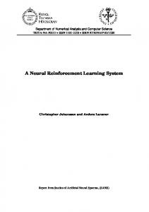
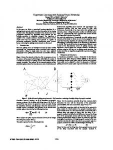
Fig. 2: 2-state model
the accuracy of approximation grows, and back-propagation search will be close to the optimal. For faster search, we use Moller’s SCG [16] that uses gradients with approximate second order derivatives. IV.
E XPERIMENTS
We examine the learning performance of nonlinear GreedyGQ by comparing it with linear Greedy-GQ and nonlinear TD. Also, we demonstrate how the correction term affects the convergence or the performance of learning. For easier analysis on the effect of the correction term, first we test a simple toy problem, consisting of 2 discrete states and actions. Next, the combination of nonlinear Greedy-GQ and continuous action control is examined on an octopus arm problem. From our pilot tests, exponential decaying 𝜖-greedy for exploration control outperformed softmax, greedy, or greedy with Gaussian noise, so the following experiments used 𝜖-greedy with quickly decreasing 𝜖 as: log 𝜖𝑁 𝜖𝑡+1 = 𝜖𝑡 × 𝑒 𝑁 , where 𝑁 is the number of episodes to train. A. 2-state model TD, linear Greedy-GQ(0) and nonlinear Greedy-GQ(0) are tested on the simple 2-state model shown in Fig. 2. The environment changes its state when an action is 1 and remains in the current state when the action is 2. The model can be summarized as follows: { 𝑠 if 𝑎 = 2 ′ 1 if 𝑠 = 2 and 𝑎 = 1 𝑠 = 2 if 𝑠 = 1 and 𝑎 = 1 { 2 if 𝑠 = 𝑎 𝑅(𝑠, 𝑎) = 1 otherwise Although this 2-state model is simple, the shape of the optimal Q function is not linear. A linear function approximation cannot cover both the state-action (1, 1) and (2, 2), and it makes hard to reach an optimal policy. Linear and nonlinear Greedy-GQ(0) were applied to the 2-state model for 1500 episodes (100 steps per each episode). This was repeated 100 times. Fig. 3 shows the mean of the 100 learning curves. From pilot tests, 𝛾 = 0.9, 𝛼 = 0.0001, and 𝛽 = 0.01 are selected for linear Greedy-GQ(0), and 𝛾 = 0.9, 𝛼𝑣 = 0.0001, 𝛼𝑤 = 0.0001, 𝛽𝑣 = 0.01, and 𝛽𝑤 = 0.001 for nonlinear Greedy-GQ(0). Here, the subscripts 𝑣 and 𝑤 represent the parameters for hidden layer and output layer respectively. Neural networks in nonlinear Greedy-GQ(0)
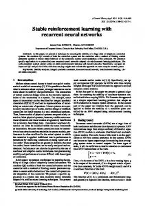
Sum of Rewards over 100 steps
185 180
nonlinear Greedy-GQ(0) linear Greedy-GQ(0) nonlinear Q-learning
175 170 165 160 155 150 145 0
200
400
600
800 Episodes
1000
1200
1400
Fig. 3: Sum of rewards per episode on 2-state model. TD (with nonlinear neural networks function approximation) and linear Greedy-GQ(0) could not find an optimal policy. For smooth curve, moving average (over 100 episodes) is used.
show the best performance with 20 hidden units. 𝜖 decays exponentially from 1 to 0.01. As shown in Fig. 3, nonlinear Greedy-GQ(0) solves what is optimized sum of rewards to the 2-state model problem, however, linear Greedy-GQ(0) is not able to learn. Linear function approximation cannot find good parameters for this 2-state problem. In Fig. 3, we can also see that nonlinear Q-learning without Greedy-GQ correction term cannot solve the problem. This means there are some factors that disturb learning. To observe this, we examine the effects of the correction terms by changing 𝛽. All combinations of 𝛽s (𝛽𝑣 , 𝛽𝑤 ∈ {0, 0.0001, 0.001, 0.01, 0.1, 0.3, 0.5, 0.7, 0.9, 0.99, 1.}) are tested and the cases with computation overflow are omitted. In Fig. 4, we observe that Q-learning without correction term (𝛽𝑣 = 𝛽𝑤 = 0) cannot learn well. Interestingly, when there is small or no correction on the hidden layer (𝛽𝑣 ≤ 0.1), it performs poorly. Correcting the gradient direction on the hidden layer is crucial for this 2-state model. In the two-layer neural networks, only the hidden layer contains a nonlinear operation, the activation function, and the output layer is linear sum of outputs from hidden units. When the target Q function is not linear, corrections in the nonlinear layer seem to be necessary for good performance. Fig. 5a shows reward versus episodes for a single run with 𝛽 = [1, 0.01]. There is a big jump in the curve around the 350th repetition. In Fig. 5b, we can see the large oscillation in TD error and its estimation, and then they drop around the 350th episode (35,000th step) as well (TD error is recorded for each state transition and 100 steps are recorded for each episode). We observe that the discrepancy from TD estimation grows in the beginning with random exploration, but as the exploration rate decreases, the TD estimation gets closer to the TD error. From this example run, Fig. 5 presents the TD gradient and Greedy-GQ(0) correction both in the hidden layer and the output layer. Unlike the output layer correction that has little effect on the gradient direction, the correction in
Fig. 4: The effects of the correction term in 2-state model. 𝑦-axis on the plot shows the sum of area under the reward curve. The 𝑥-axis is sorted by 𝛽𝑣 and 𝛽𝑤 . The yellow area groups the results with 𝛽𝑣 ≤ 0.1, and the rest shows the results with 𝛽 ≥ 0.5. For 10 runs, small learning rates 𝛽𝑣 for the hidden layer result in lower performance.
the hidden layer has a large impact on the gradient. When the TD error hits the maximum, and at the same time when the learning curve jumps up, the correction term modifies the gradient direction to reduce the TD error and eventually leads to an optimal policy. B. Octopus Arm A real octopus arm is a complex organ with many degrees of freedom. Here, the Yekutieli’s two-dimensional model [25] is used. The model is composed of spring muscles for each compartment. The basis of the model is that muscular hydrostats maintain a constant volume [8], so forces are transferred among the segments. Gravity, buoyancy, fluid friction, internal particle repulsion and pressure, and muscle contractions are computed each time step. For our experiments, we used the octopus arm model in the RL-competition [4] (Fig. 6). The problem contains 10 compartments, and the ventral, dorsal, and transverse muscles are controlled by independent activation variables. To make the problem simple, Engel, et al., [7] used 6 predefined discrete actions. In this paper, without reducing the action space, we train the arm to learn from the full action space defined by 33-dimensional real-valued actions. For the 10-compartment example, the state space is defined by 82 continuous values: base angle, angular
velocity, x-y coordinate positions of each joints, and their velocities. We place the goal at (4, 3) as in Fig. 6. Initially the base of the arm is placed close to (0, 0) and the arm is straight toward the right. The target task is touching the goal with any part of the arm. On each time step, the arm receives −0.01 as a penalty, and if it reaches the goal, it gets 10 as a reward. The maximum number of steps per each episode is limited to 1000 steps. Thus, if the arm touches the goal at the last moment, the total reward will be 0. If it fails to reach the goal, the total will be −10. Positive, larger rewards are obtained when the goal is reached sooner. The episodes are repeated 500 times with exponentially decreasing 𝜖 value from 1 to 0.01. From pilot tests, 𝛼 = [0.0001, 0.0001] is selected. Each experiment was run 10 times. Among all 𝛽 combinations, 𝛽 = [0.1, 0.0001] shows the best performance and less variation than other 𝛽 values. From this, as we examined in previous section, we can verify the stability contribution of the correction term empirically. Fig. 7 compares the performance between continuous and discrete actions. After failing to touch the goal in the beginning, continuous control finds sequences of continuous actions that result in reaching the goal. With 6 discrete actions, it fails to reach the goal in 500 repetitions. It may need more
150
190
100
180
50
170
0
TD error
Rewards
200
160
50
150
100
140
150
130 0
200
400
600
800
episodes
1000
1200
1400
TD error estimated (φT g)
200 0
20000
40000
60000
80000 100000 120000 140000 steps
(a) Examplar learning curve
(b) TD error (𝛿) and approximation (𝛿𝑘 𝑔𝑤𝑘 ) in Greedy-GQ(0)
(c) TD gradient (hidden)
(d) Greedy-GQ(0) correction (hidden)
(e) TD gradient (output)
(f) Greedy-GQ(0) correction (output)
Fig. 5: TD gradient and Greedy-GQ(0) correction term in hidden and output layer
10
1000
sum of rewards
600 0 400 5
100
(a) Initial position
# of steps
800
5
200
100
200
episodes
300
400
5000
(a) Continuous actions
10
1000
sum of rewards
600 0 400 5
(b) Controlling the arm
Fig. 6: Benchmark octopus arm control problem
100
# of steps
800
5
200
100
200
episodes
300
400
5000
(b) 6 discrete actions
experience to learn the policy to touch the goal. Although it is not presented, Q-learning(0) with or without continuous action search has been tested, but a positive learning curve was never observed, indicating further experience may be needed. Only nonlinear Greedy-GQ(0) with continuous actions was able to solve the task. Reviewing the state trajectories, we also found that with discrete actions, the arm failed to find the short sequence of anti-clockwise movements towards to the goal. It only experienced clock-wise rotation to reach the goal, which costs more than 850 steps. Continuous action provides the additional flexibility during the early exploration stage to find the shorter paths of less than 200 steps. The number of steps in Fig. 7 shows this as well: continuous action (Fig. 7a) shows various experience that reaches to the goal in a wide range of steps, but discrete action (Fig. 7b) limits the experience to paths of more than 600 steps. V.
C ONCLUSION
This paper extends linear Greedy-GQ to a nonlinear form with feed-forward neural networks for stable learning performance and then combines it with continuous action search. An
Fig. 7: Performance comparison between continuous action and discrete action control. Thick lines show the sum of rewards and dash lines show the number of steps per each episode. TD(0) fails to learn in 500 repetitions, so the learning curve is omitted.
analysis reveals that the nonlinear Greedy-GQ correction term is crucial for training the hidden layer when the target Q function is nonlinear. Testing on a complex octopus problem with a high dimensional continuous domain, we observe that the continuous action search improves the learning performance (both in speed and asymptotic level). Future research activity will follow in three main directions: examining more realworld problems, applying Regularized Off-Policy TD learning (RO-TD) [11] to be robust to noisy inputs, and development of batch-oriented version of nonlinear Greedy-GQ and comparative research against other state-of-the-art algorithms such as CACLA [24] and SMC-learning [3]. R EFERENCES [1] L. Baird. Residual algorithms: Reinforcement learning with function approximation. In Proceedings of 12th International Conference on
Machine Learning, pages 30–37, 1995. [2] H. Benbrahim and J. A. Franklin. Biped dynamic walking using reinforcement learning. Robotics and Autonomous Systems, 22(3):283– 302, 1997. [3] A. L. M. R. A. Bonarini. Reinforcement learning in continuous action spaces through sequential monte carlo methods. Proc. Adv. Neural Inf. Process. Syst, 20:833–840, 2008. [4] R. Community. Rl-competition. http://www.rl-competition.org/, 2009. [Online; accessed 03-July-2014]. [5] T. Degris, M. White, and R. S. Sutton. Off-policy actor-critic. arXiv preprint arXiv:1205.4839, 2012. [6] M. Dorigo and M. Colombetti. Robot shaping: Developing autonomous agents through learning. Artificial intelligence, 71(2):321–370, 1994. [7] Y. Engel, P. Szabo, and D. Volkinshtein. Learning to control an octopus arm with gaussian process temporal difference methods. Advances in Neural Information Processing Systems, 18:347, 2006. [8] W. M. Kier and K. K. Smith. Tongues, tentacles and trunks: the biomechanics of movement in muscular-hydrostats. Zoological Journal of the Linnean Society, 83(4):307–324, 1985. [9] J. Z. Kolter. The fixed points of off-policy td. pages 2169–2177, 2011. [10] L.-J. Lin. Self-improving reactive agents based on reinforcement learning, planning and teaching. Machine learning, 8(3-4):293–321, 1992. [11] B. Liu, S. Mahadevan, and J. Liu. Regularized off-policy td-learning. pages 845–853, 2012. [12] H. R. Maei. Gradient temporal-difference learning algorithms. PhD thesis, University of Alberta, 2011. [13] H. R. Maei, C. Szepesv´ari, S. Bhatnagar, D. Precup, D. Silver, and R. S. Sutton. Convergent temporal-difference learning with arbitrary smooth function approximation. pages 1204–1212, 2009. [14] H. R. Maei, C. Szepesv´ari, S. Bhatnagar, and R. S. Sutton. Toward offpolicy learning control with function approximation. In Proceedings of the 27th International Conference on Machine Learning, pages 719– 726, 2010. [15] J. D. R. Mill´an, D. Posenato, and E. Dedieu. Continuous-action qlearning. Machine Learning, 49(2-3):247–265, 2002. [16] M. Møller. A scaled conjugate gradient algorithm for fast supervised learning. Neural networks, 6(4):525–533, 1993. [17] J. Santamaria, R. Sutton, and A. Ram. Experiments with reinforcement learning in problems with continuous state and action spaces. Adaptive behavior, 6(2):163, 1997. [18] P. Stone and R. S. Sutton. Scaling reinforcement learning toward robocup soccer. In In International Conference on Machine Learning, volume 1, pages 537–544, 2001. [19] P. Stone, R. S. Sutton, and G. Kuhlmann. Reinforcement learning for robocup soccer keepaway. Adaptive Behavior, 13(3):165–188, 2005. [20] R. Sutton and A. Barto. Reinforcement Learning: An Introduction. The MIT press, 1998. [21] R. S. Sutton, H. R. Maei, D. Precup, S. Bhatnagar, D. Silver, C. Szepesv´ari, and E. Wiewiora. Fast gradient-descent methods for temporal-difference learning with linear function approximation. In Proceedings of the 26th Annual International Conference on Machine Learning, pages 993–1000, 2009. [22] V. Tadi´c. On the convergence of temporal-difference learning with linear function approximation. Machine Learning, 42(3):241–267, 2001. [23] J. N. Tsitsiklis and B. Van Roy. An analysis of temporal-difference learning with function approximation. Automatic Control, IEEE Transactions on, 42(5):674–690, 1997. [24] H. Van Hasselt and M. A. Wiering. Reinforcement learning in continuous action spaces. In Approximate Dynamic Programming and Reinforcement Learning, 2007. IEEE International Symposium on, pages 272–279, 2007. [25] Y. Yekutieli, R. Sagiv-Zohar, R. Aharonov, Y. Engel, B. Hochner, and T. Flash. Dynamic model of the octopus arm. i. biomechanics of the octopus reaching movement. Journal of neurophysiology, 94(2):1443– 1458, 2005.