International Journal of Computer and Electrical Engineering, Vol. 1, No. 5 December, 2009
1793-8163
A New Algorithm for Voice Signal Compression (VSC) and Analysis Suitable for Limited Storage Devices Using MatLab Shiv Kumar, Member IACSIT, Vijay K Chaudhari, Member IACSIT, Dr. R. K. Singh, Dr. Dinesh Varshney
Abstract- This research work reveals that Voice Signal Compression (VSC) is a technique that is used to convert the voice signal into encoded form when compression is required, it can be decoded at the closest approximation value of the original signal. This work presents a new algorithm to compress voice signals by using an “Adaptive Wavelet Packet Decomposition and Psychoacoustic Model”. The main goals of this research work is to transparent compression (48% to 50%) of high quality voice signal at about 45 kbps with same extension (i.e. .wav to .wav), second is evaluate compressed voice signal with original voice signal with the help of distortion and frequency spectrum analysis and third is to compute the signal to noise ratio (SNR) of the source file.For this, a filter bank is used according to psychoacoustic model criteria and computational complexity of the decoder. The bit allocation method is used for this which also takes the input from Psychoacoustic model. Filter bank structure generates quality of performance in the form of subband perceptual rate which is computed in the form of perceptual entropy (PE). Output can get best value reconstruction possible considering the size of the output existing at the encoder. The result is a variable-rate compression scheme for high-quality voice signal. This work is well suited to high-quality voice signal transfer for Internet and storage applications. Index Terms- Matlab6.5, Wavelet Toolbox, Psychoacoustic Model, Algorithm
I.
milliseconds. If one tone [22] is masking another, the effect depends on the separation in frequency. Fig. - [1] shows a typical plot of the masking effect (for example, for plots of maskers at different frequencies) [1], [7], [12], [15]. The solid black line is the threshold of audibility. A spectral component on the left causes the threshold of audibility to be shifted upward, shown by the dotted line. In Fig. -[1], the threshold of auditory (solid line) shifted in the presence of a masker (left arrow). A second spectral component, shown by the arrow on the right, is masked. Notice that the masking effect falls off more steeply to the right of the curve, that is, toward higher frequencies, but a higher tone affects relatively mask more high frequencies, but a high tone affects relatively fewer lower frequencies. Masking may also happen if the tones are not simultaneous; i.e. if masking tone is short but occurs before another tone, the masked tone can still be obscured. Masking effect happens whether the masker is a single tone or a broader band of noise. Laboratory studies of such masking effects led to the notion of critical band; i.e. a given frequency is surrounded by a band of frequencies within which various auditory phenomena can be shown to occur. For example, consider the loudness percept evoked when two tones are at the same frequency.
INTRODUCTION
Masking may be easier to explain the visual domain. If a bright light is shinning in our eyes, such as headlights from an oncoming car, then other dimmer lights are impossible to see. There are similar phenomena in the auditory world. One sound can make it impossible to hear another or one sound may shift the apparent loudness of another. The masking of one sound may be total or partial. Also, parts of one sound can mask parts of another sound, even if we cannot consciously detect such masking in normal circumstances. Auditory masking effects can die away in a matter of Manuscript received June 28, 2009. Shiv Kumar is with Department of Information Technology, Technocrat Institute of Technology-Bhopal (M.P.)-India (Mobile No.: +919827318266, e-mail:
[email protected]). Asst. Prof. Vijay K Chaudhari is Department of Information Technology, Technocrat Institute of Technology-Bhopal (M.P.)-India (Mobile No.: +91-9893181833-e-mail:
[email protected]). Dr. R.K. Singh is Director, MATS University, Raipur (C.G.), India. (Mobile No.: +91-9893623490, e-mail:
[email protected]). Dr. Dinesh Varshney is with Multimedia Research Department, Multimedia regional centre, Madhya Pradesh Bhoj (Open) University, Khandwa road Campus, Indore (M.P.)-India (Mobile No.: +91-9826076903 email:
[email protected])
[Fig. - 1: The Threshold of Audibility (Solid line) Shifted in the Presence of a Masker (left arrow)]
Is selected voice signal may be hear by human nervous system or not? It can be checkout by psychoacoustics model [5], [7], [8], [9], [10], [14], [16], [17], [18], [21], [22]. Those signal has frequency in between 20Hz to 20KHz is called tone that take major responsibility in the computation 656
International Journal of Computer and Electrical Engineering, Vol. 1, No. 5 December, 2009
1793-8163 of voice signal that define which signal can be heard by human nervous system and which is not. Voice signals first break in the pre-defined frames (2048 bytes) and then tone computation is done on the basis of each frame that is masked after tone computation. First turn to the interaction between physical stimuli and the human nervous system. For this discussion, voice is defined as a disturbance in air pressure that reaches the human eardrum. In terms of frequency, amplitude, time, and other parameters, there are limits to the kinds of air pressure disturbance that will evoke an auditory percept in humans. The development of the human ear’s limitation and capabilities was undoubtedly motivated by evolutionary necessity. Survival is granted to those who can distinguish the rustle of an attacker in a forest, for example, from a babbling brook nearby. As we know that sound is audible (hearing) for humans in a range from 20 Hz to 20 KHz can be broken up into critical bandwidths, which are non-uniform, non-linear, and dependent on the heard sound [12], [15]. Signals within one critical bandwidth are hard to separate for a human observer. It is found that the frequency range from 20 Hz to 20 kHz can be broken up into critical bandwidths, which are nonuniform, non-linear, and dependent on the level of the incoming sound. Signals within one critical bandwidth are hard to separate for a human observer. The center frequency location of these critical sub-bands is known as the critical band rate and approximately follows the expression equation (2) (Described in the Bark scale and Fletcher curves).
Z = [ A1 + A2 ]bark .....(2)
Where
A. Absolute Threshold of hearing (ATH) The absolute threshold of hearing (ATH), or threshold in quiet (Tq), is the average sound pressure level (SPL) below in equation (1) in which human ear does not detect any stimulus [20]. f f 4 -0.6*(( )-3.3)2 3*( ) f -0.8 T q (f) = 3.64*( ) -6.5e 1000 +10 1000 ....(1) 1000
Where f is frequency in Hertz, Tq is threshold in dB. Signal can take a leap for the purposes of compression, if a signal has any frequency components with power levels that fall below the absolute threshold of hearing, and then these components can be discarded, as the average listener will be unable to hear those frequencies of the signal anyway. Auditory masking is a perceptual property of the human auditory system that occurs whenever the presence of a strong audio signal makes a temporal or spectral neighborhood of weaker audio signal imperceptible. Normally they are studied separately and known as simultaneous masking and temporal masking. If two sounds occur simultaneously and one is masked by the other, this is referred to as simultaneous masking that is mentioned in fig.-[3]. If a signal has any frequency components with power levels that fall below the absolute threshold of hearing, then these components can be discarded as the average listener will be unable to hear those frequencies of the signal anyway. Similarly, a weak sound emitted soon after the end of a louder sound is masked by the louder sound. In fact, even a weak sound just before a louder sound can be masked by the louder sound. These two effects are called forward and backward temporal masking; respectively that is mention in fig.-[4].
A1 = 13*arctan(0.00076* Hz ) A2 = 3.5arctan(( f ) 2 ) 7500
The distance from one critical band center to the center of the next band is 1 Bark. The human auditory frequency range spreads from 20 Hz to 20 KHz and covers approximately 25 Barks. General frequency response [20] is mention in fig.-[2].
B. Auditory Masking Humans do not have the ability to hear minute differences in frequency. This becomes even more difficult if the two signals are playing at the same time. For a masked signal to be heard, its power will need to be increased to a level greater than that of a threshold that is determined by the frequency of the masker tone and its strength. It turns out that noise can be a masker as well. If noise is strong enough, it can mask a tone that would be clear otherwise. In a compression algorithm, therefore, one must determine: (i). Tone Maskers Determining whether a frequency component is a tone (Masker) requires knowing whether it has been held constant for a period of time, as well as whether it is a sharp peak in the frequency spectrum, which indicates that it is above the ambient noise of the signal. A frequency f (with FFT index k) is a tone if its power spectral P[k] [4] is:
[Fig.-2: Psychoacoustic Critical Band]
Two main properties of the human auditory system that make the psychoacoustic model [4], [7], [17], [19], [20] are:
§ Greater than P [k+1] and P [k-1], i.e. the neighborhood is [k-2 …. K+2].
657
International Journal of Computer and Electrical Engineering, Vol. 1, No. 5 December, 2009
1793-8163 § 7 dB greater than other frequencies in its neighborhood, where the neighborhood is dependent on f: • If 0.17 Hz < f < 5.5 kHz, the neighborhood is [k2…k+2] • If 5.5 kHz ≤ f < 11 kHz, the neighborhood is [k3…k+3] • If 11 kHz ≤ f < 20 kHz, the neighborhood is [k6…k+6]
For noise
The Spreading Function is defined in table-II. Where ∆z =z(i)-z(j), SF(i, j) is spreading function [Table-II: Spreading Function]
SF(i, j) =
II.
17∆z - 0.4Ptm(j) + 11
-3 ≤ ∆z < -1
∆z(0.4Ptm(j) + 6)
-1 ≤ ∆z < 0
-17∆z
0 ≤ ∆z < 1
∆z(0.15Ptm(j) - 17) – 0.15Ptm(j)
1 ≤ ∆z < 8
LITERATURE SURVEY AND PROBLEM IDENTIFICATION
There is an explanation of different technique for wavelet compression in which speech processing for compression and recognition was addressed [1]. Various methods and paradigms based on the time-frequency and time-scale domains representation for the purpose of compression and recognition were discussed along with their advantages and draw-backs. Level dependent and global threshold compression schemes were also examined in details. Work was good but wavelet family is not defined means which wavelet family was used for data compression, how much data was compressed, and what was file extension after compression? According to this previous work [1], work is further extended practically where dubechies wavelets family is used with transparent compression of high quality voice signal at about 45 kbps. Selected .wav file is compressed 48% to 5o% of the source file with same extension (i.e. .wav to .wav). In the work [2], a technique was presented for image compression by using lossy compression. The methods were applied to the Vocational Training School (T.E.E.) in the Greek Education System for teaching aspects related to networks and image compression using MatLab Language. The effectiveness of the approach was evaluated by comparing the performances of the sample students and comparing the outcomes with those of a traditional teaching approach. The encoding of coefficients is done using runlength-encoding of the zeros. Whole work is done only and only for image compression and after compression analysis was done to selected network. This work [2] was good but after compression file extension is changed. What would happen if we want to compress the file without changing the extension? This work is further extended in which after compression file extension is same as source file (i.e. .wav to .wav). In the research [3], describes the performance of different types of wavelets for composing the transient audio signal. The wavelets that were investigated for this purpose are dubechies family of wavelets, wavelet packets and multiwavelets. The performances of various wavelets are compared, based on compression ratio and the signal to noise ratio (SNR) value of the reconstructed signal. One of the main challenges to the application of multi-wavelets is the problem of multi-wavelet initialization (or better known as pre-filtering). In the case of scalar wavelets, the given signal data is usually assumed to be the scaling coefficients
[Fig.-3: Simultaneous Masking]
[Fig.-4: Temporal Masking] (ii). Noise Maskers If a signal is not a tone, it must be noise. Thus, one can take all frequency components that are not part of a tone neighborhood and treat them like noise. (iii). Masking Effects The maskers which have been determined affect not only the frequencies within a critical band, but also in surrounding bands. The spreading can be described as a function SF(i, j) that depends on the maskee location i, masker location j, the power spectrum (Ptm) at j, and difference between masker and maskee locations in Barks. As a result, the masks can be modeled same variables as defined in table-I. [Table-I: Tone and Noise] For tones
Pnm(j) - 0.175z(j) + SF(i, j) - 2.025 (dB SPL)
Ptm(j) - 0.275z(j) + SF(i, j) - 6.025 (dB SPL)
658
International Journal of Computer and Electrical Engineering, Vol. 1, No. 5 December, 2009
1793-8163 that are sampled at a certain resolution, and hence, multiresolution decomposition can directly be applied on the given signal. Unfortunately, the same technique cannot be employed directly in the multi-wavelet setting. Some preprocessing has to be performed on the input signal, prior to multi-wavelet decomposition. In this implementation work [3] that was based on multi-wavelet, give good results in comparison to the daubechies bases. On the basis of the experimentation presented, it can therefore be concluded that multi-wavelets, with an appropriate choice of prefiltering method, seem to represent a promising substitute for scalar wavelets in audio data compression problems. In this paper [3], how can analyze that recorded signals are audible? How can analyze that recorded signals are in the range of human nervous system? The quality of signal is calculated by acoustic model which is not defined in this paper [3]. Quantization is done to achieve better compression that reduces the number of bits needed to store information by reducing the size of the integers representing the information in the scene. These are the details that the human visual system ignores. This step represents one key segment in the multi-compression process. A reduction in the number of bits reduces storage capacity needed, improves bandwidth, and lowers implementation costs. In the paper [3], level of quantization (8-bit, 16-bit, etc...) and threshold techniques is not defined. According to this previous work [3], work is further extended in which psychoacoustic model is used to compute which recorded signal belongs to human nervous system. To do this hard and global threshold is used. For better compression, 16-bit dynamic quantization (narrow range quantization) is used. As mentioned in work [6], voice recognition technology can be used as a more efficient in car security system. Now if voice recognition is done by .wav file then it can be better but if voice recognition is done by compressed .wav file then it will be best. To get compressed .wav file, this work is beneficial. According to research [22], the current data reveal that sensitivity to tonality changes significantly across the tessitura, with dramatically reduced sensitivity to tonality in lower pitch regions and moderately reduced tonality perception in upper pitch regions. Such an asymmetric sensitivity function may result from the combined influence of pitch salience (or a co-varying factor such as exposure to pitch distributional information in music) and reduced pitch processing that occurs when inharmonic levels exceed the threshold of detection. In this previous work [22], if tonality is computed then further work compression is possible which is done in this research work VSC. III. PROPOSED SOLUTION
Step-7: Calculate power spectrum density Step-8: Calculate the tonality Step-9: If selected voice signal is a tone then go to next step otherwise exit Step-10: Compute energy of the tone Step-11: Compute entropy of the tone Step-12: Compute SNR of the tone Step-13: Evaluation of Distortion Computation Step-14: Define wavelet compression scheme Step-15: Define quantization level Step-16: Compute offset to shift memory location of entire partition Step-17: Reconstructs the signal based on the multilevel wavelet decomposition structure Step-18: Define wavelet expander scheme for reconstructed signal Step-19: Write expanded .wav file (compressed file) B. Block Diagram of VSC Wavelet decomposition is done on selected (input) voice signal and then adaptive wavelet compression scheme is defined. At the same time tone computation is done with the help of psychoacoustic model and Fast Fourier Transform (FFT) of same selected voice signal. Now if signal is tone, then bit allocation is performed that produce stream of data which is defined in fig.-[5(a)]. Now this stream of data is reconstructed which is defined in fig.[5(b)].
Wavelet Decomposition
Input
FFT (Frame Size)
Wavelet Compression Psychoacoustic Model
Bit Allocation
Header Stream of Data
ENCODER
Fig.:-5(a): Block Diagram of VSC for Encoder Stream of Data
Header Extraction
Wavelet Reconstruction Output (.wav File)
DECODER Fig.:-5(b): Block Diagram of VSC for Decoder
A. Approach The approach for VSC is defined in following steps: Step-1: Select wavelet functions Step-2: Load the recorded voice signal Step-3: Define Decomposition levels = N Step-4: Break the voice signal into N frame Step-5: Define wavelet coefficients Step-6: Compute the masking thresholds
C. 0-Level DFD of VSC Input
Recorded Voice Signal
VSC
Compressed Voice Signal
Fig.-6: 0-Level DFD of VSC
659
Output
International Journal of Computer and Electrical Engineering, Vol. 1, No. 5 December, 2009
1793-8163 D. Flow Chart of VSC START Where Coefficients: file=recorded voice signal C = wavelet decomposed frame L = Length of coefficient C n = number of bits required for quantization level P = Power Density Ptm = Power Spectral Density of Tone Masker E = Entropy SNR = Signal to Noise Ratio xd = compressed file
Define Wavelet Function(x) Level = 5 Wavelet = dB10 frame_size =2048 file= ‘SAMPLE1.wav’ [x,Fs,bits] = wavread(file) xlen=length(x) Step =frame_size N=ceil (xlen/step)
Cchunks=0; Lchunks=0; Csize=0; PERF0mean=0; PERFL2mean=0; n_avg=0; n_max=0;
n_0=0; n_vector=[];
i=1:1: N No
i==N
Yes
frame= x([(step*(i-1)+1):step*i])
frame= x([(step*(i-1)+1):length(x)])
[C, L] = wavedec(frame, level, wavelet) Yes
No
Wavelet_Compression==0
thr=thr*10^6 [thr, sorh, keepapp] = ddencmp('cmp', 'wv', frame)
[XC, CXC, LXC, PERF0, PERFL2] = wdencmp('gbl', C, L, wavelet, level, thr, sorh, keepapp) C=CXC L=LXC PERF0mean= PERF0mean + PERF0 PERFL2mean= PERFL2mean+PERFL2 Yes
Psychoacoustic==on
No
P=10.*log10 ((abs (fft (frame, length (frame)))). ^2) Ptm= zeros (1, length (P)) k= 1: 1: length (P) No
(K≤1)│ (k≥ 250)
Yes
bool=0
B1 A1
[Fig.-7(a): Flow Chart of VSC] 660
International Journal of Computer and Electrical Engineering, Vol. 1, No. 5 December, 2009
1793-8163
A1
No
B1
Yes
P(k)2) & (k(P(k-2)+7)) & (P(k)>(P(k+2)+7))) Yes
(K≥63) & (k(P(k-2)+7)) & (P(k)>(P(k+2)+7)) & (P(k)>(P(k-3)+7)) & (P(k)>(P(k+3)+7))) Yes
bool = ((P(k)>(P(k-2)+7)) & (P(k)>(P(k+2)+7)) & (P(k)>(P(k-3)+7)) & (P(k)>(P(k+3)+7)) & (P(k)>(P(k-4)+7)) & (P(k)>(P(k+4)+7)) &(P(k)>(P(k-5)+7)) & (P(k)>(P(k+5)+7)) & (P(k)>(P(k-6)+7)) &(P(k)>(P(k+6)+7))) bool==1 Yes
No
(k>=127) & (k≤ 256) No bool=0
No
Ptm(k)= 10*log10(10.^(0.1.*(P(k-1)))+10.^(0.1.*(P(k)))+10.^(0.1.*P(k+1)))
Sum_energy=0 k=1:1:length(Ptm) sum_energy=10.^(0.1.*(Ptm(k)))+sum_energy E=10*log10(sum_energy/(length(Ptm))) SNR=max (P)-E n=ceil (SNR/6.02) Yes
n≤3
n=4 n_0=n_0+1
No n≥n_max Yes n_max=n
n_avg=n+n_avg; n_vector=[n_vector n] compander=on
No
Yes Mu=255 C = compand(C, Mu, max(C), 'mu/compressor') quantization =on psychoacoustic=off
No
Yes n=8 partition = [min(C):((max(C)-min(C))/2^n):max(C)] codebook = [min(C):((max(C)-min(C))/2^n):max(C)] [index, quant, distor] = quantiz(C, partition, codebook) A2 B2
[Fig.-7(b): Flow Chart of VSC]
661
International Journal of Computer and Electrical Engineering, Vol. 1, No. 5 December, 2009
1793-8163
A2
B2
Offset=0 j=1: 1: N C(j)=0 Yes offset=-quant(j) quant=quant +offset C=quant Cchunks=[Cchunks C] Lchunks=[Lchunks L] Csize=[Csize length(C)] Encoder = round((i/N)*100) Cchunks=Cchunks(2:length(Cchunks)) Csize=[Csize(2) Csize(N+1)] Lsize=length(L) Lchunks=[Lchunks(2:Lsize+1) Lchunks((N-1)*Lsize+1:length(Lchunks))] PERF0mean=PERF0mean/N PERFL2mean=PERFL2mean/N n_avg=n_avg/N n_max;
Encoding Completed
xdchunks=0 i=1:1:N No
i==N
Yes
Cframe=Cchunks([((Csize(1)*(i-1))+1):Csize(2)+(Csize(1)*(i-1))]) Cframe=Cchunks([((Csize(1)*(i-1))+1):Csize(1)*i])
Compander=on max(Cframe)=0 Yes Cframe = compand(Cframe,Mu,max(Cframe),'mu/expander')
Compander=on max(Cframe)=0 Yes Cframe = compand(Cframe,Mu,max(Cframe),'mu/expander')
xd = waverec(Cframe,Lchunks(Lsize+2:length(Lchunks)),wavelet)
xd = waverec(Cframe,Lchunks(1:Lsize),wavelet) xdchunks=[xdchunks xd]
Decoder = round((i/N)*100) xdchunks=xdchunks(2:length(xdchunks)) distorsion = sum(('xdchunks-x').^2)/length(x)
wavwrite(xdchunks,Fs,bits)
STOP
[Fig.-7(c): Flow Chart of VSC] 662
Decoding Completed Plot Figure of source and compressed file
International Journal of Computer and Electrical Engineering, Vol. 1, No. 5 December, 2009
1793-8163 IV.
PROPOSED SOLUTION
This result analysis is done by IBM Intel P4, 3.0 GHz Processor, 256 MB RAM, 40 GB Hard Disk, and WindowsXP Service Pack-2 Operating System and MAtLab7.0. Age factor define the clarity in audible voice and SNR. In this result analysis, I take five samples, three samples belong to male category and two samples belong to female category. Where n = number of bits required for quantization, SNR = Signal to Noise Ratio. A. Result Analysis for Male and Female Category Voice Signal The result analysis for male category voice signal is taken from Sample1.wav, Sample3.wav, and Sample5.wav and for female category voice signal is taken from Sample2.wav, Sample6.wav in which voice recording is done for different sentences. Each sample belongs to different age category and different environment also. Result analysis summary for male and female category voice signal is mention in Table[III]. Similarly frequency spectrum for Sample1.wav, Sample2.wav, sample3.wav, Sample5.wav, and Sample6.wav are shown in fig.-[8(a)], fig.-[8(b)], fig.-[8(c)], fig.-[8(d)], and fig.-[8(e)] respectively where spectrum for each selected file clearly defines the difference between source file & compressed file. The difference is computed on the basis of amplitude and time (or frequency) response of selected and compressed file.
Fig.-8(c): Frequency Spectrum Before and After Compression for Sample3.wav
Fig.-8(d): Frequency Spectrum Before and After Compression for Sample5.wav
Fig.-8(e): Frequency Spectrum Before and After Compression for Sample6.wav
V.
IMPLEMENTATION DETAILS
To compute the tone, first computation is done for power spectral density (P). P = 1 0 lo g
10
((a b s (fft(fra m e , le n g th (fra m e ))))
2
The tone masker checks the power spectrum p at index k and returns a boolean indicating whether it is a tone. If p(k) is a local maxima and is greater than 7db in a frequency dependent neighborhood, it is a tone. This neighborhood is defined as: Within 2: if 2(P(k-2)+7))&(P(k)>(P(k+2)+7))& (P(k)>(P(k-3)+7)) & (P(k)>(P(k+3)+7))); For within 2, 3, 4, 5, and 6 neighborhood: Fig.-8(b): Frequency Spectrum Before and After Compression for Sample2.wav
663
International Journal of Computer and Electrical Engineering, Vol. 1, No. 5 December, 2009
1793-8163 bool
=
REFERENCES
((P(k)>(P(k-2)+7)) & (P(k)>(P(k+2)+7)) & (P(k)>(P(k-3)+7)) & (P(k)>(P(k+3)+7)) & (P(k)>(P(k-4)+7)) & (P(k)>(P(k+4)+7)) &(P(k)>(P(k-5)+7)) & (P(k)>(P(k+5)+7)) & (P(k)>(P(k-6)+7)) &(P(k)>(P(k+6)+7)));
[1]
[2]
If selected signal is a tone then there is need to compute power spectral density of tones masker (Ptm): Ptm(k) = 10log
10
(10
0.1(P(k-1))
VI.
+ 10
0.1(P(k))
+ 10
0.1(P(k+1))
)
[3]
[4]
CONCLUSION
[5]
On the basis of Daubeshies (db10) wavelet family, Adaptive wavelet packet decomposition and psychoacoustic model compression is done approximately 48% to 50% of source file. In the whole work, it is found that every recorded voice contains energy that displays average information (Entropy). For each frame of recorded voice, SNR is computed from the entropy. During the computation of tone, frame size is decided 2048 bits for decomposition. To mask lower signal with upper signal, threshold masking technique is used. All decomposed frames are again reconstructed with 16-bit quantization scheme to get better compression result. This work is useful for limited storage devices (Pervasive Computing) and Global transmission medium. VII.
[6]
[7]
[8]
FUTURE WORK
[9]
From the collected data, findings are that there is long way to compete other compression schemes like mp3, .mp4, .avi….etc. There is need to increase the compression ratio which is under the development. Analysis for different parameters (i.e. Single Eco, Multiple Eco, Fade-In, Fade-Out, Pitch Low, Pitch High, FIR Reverb, IIR Reverb, Flat Response...etc) of this compressed voice signal is also possible for the purpose of security or voice signal identification which under the research.
[10]
[11]
ACKNOWLEDGMENT First my greatest thank goes to God, bright morning stars and authors of life. I would like to express my sincere and earliest thanks to my guide hardworking, enduring, and kindhearted person Prof. Vijay K Chaudhari (Head, Department of Information Technology), Dr. R.K. Singh (Director, MATS University- Raipur(C.G.)-India), and Dr. Dinesh Varshney (Regional Director, Madhya Pradesh Bhoj University-Indore-India for his kind guidance throughout this research and under whom I am able to do successfully. I extend my heart-felt thank to Prof. Mohd. Ilyas Khan (Assistant Professor, Department of Information Technology) for his kind support during design DFD, and Flow Chart. This work would not have progressed without his kind support. I express my ardent and earnest gratitude to my spouse Dr. Shachi Sahu (Sr. Lecturer, Departmet of Applied Chemistry, TITE-Bhopal) for her motivation, ardent encouragement, supports, and helps during making this research work. Really without her support, I could not do it.
[12]
[13] [14]
[15] [16]
[17]
[18]
664
Jalal Karam, "Various Speech Processing Techniques For Speech Compression And Recognition", proceedings of world academy of science, engineering and technology volume 26 December 2007 ISSN 1307-6884, © 2007 waset.org http://www.waset.org/pwaset/v26/v26-133.pdf Sarantos Psycharis “The Didactic Use Of Digital Image Lossy Compression Methods For The Vocational Training Sector”, University of Agean, Proceeding of Current Developments in Technology-Assisted Education 2006(FORMATEX 2006) http://www.formatex.org/micte2006/pdf/2065-2069.pdf P R Deshmukh, "Multi-wavelet Decomposition for Audio Compression", IE(I) Journal-ET, Vol 87 , July 2006 http://www.ieindia.org/pdf/87/mem06915.pdf Background on the Psychoacoustic Model “W.A.V.S. Compression” http://is.rice.edu/~welsh/elec431/psychoAcoustic.html Stefan Wabnik, Gerald Schuller, Ulrich Kr amer and Jens Hirschfeld, “Frequency warping In Low delay Audio Coding”, ICASSP 2005, 07803-8874-7/05/$20.00 ©2005 IEEE www.idmt.fraunhofer.de/de/geschaeftsfelder/schuller/ic assp05_0300181.pdf Shaleena Jeeawoody, “Voice Analysis and Recognition as a Car Theft Deterrent”, California State Science Fair 2008, Project No: J1307, Ap2/08 http://www.USC.edu/CSSF/Current/Projects/J1307.pdf Pavel Rajmic and Jan Vlach, "Real-Time Audio Processing Via Segmented wavelet Transform" Proc. of the 10th Int. Conference on Digital Audio Effects (DAFx-07), Bordeaux, France, September 1015, 2007 http://dafx.labri.fr/main/papers/p055.pdf Hongwu YANG, Dezhi HUANG, Lianhong CAI, “Perceptually Weighted Mel–Cepstrum Analysis Of Speech Based On Psychoacoustic Model”, IEICE TRANS. INF. & SYST., VOL.E89-D, No.12 December 2006 http://hcsi.cs.tsinghua.edu.cn/Paper/paper06/200601.pdf Samar Krimi, Kais Ouni, Noureddine Ellouze, “Realization of a Psychoacoustic Model for MPEG-1 using Gammachirp WaveLet”, Proceeding in EUSIPCO,2005 http://www.eurasip.org/Proceedings/Eusipco/Eusipco2005/defevent/p apers/cr1936.pdf Tsung-Han Tsai, Yi-Wen Wang, Shih-Way Hung “An MDCT-Based psychoacoustic model co-processor design for MPEG-2/4 AAC audio encoder” Proceeding in the 7th International Conference on Digital Audio Effects (DAFx’04), Naples, Italy, October 5-8, 2004 http://www.mp3-tech.org/programmer/docs/P_335.pdf Ganesh K Venayagamoorthy, Viresh Moonasar, Kumbes Sandrasegaran, “Voice Recognition Using Neural Networks”,Institute of Information Science and Technology (IIST), Massey University, New Zealand, Published in IEEE in 1998, Val. No. 0-7803-50545.0029 http://acil.mst.edu/documents/voice_recognition_using.pdf Andress Holzinger with assistance from G. Searle, “Multimedia Basics”, Volume 1: Technology, ISBN: 81-7008-243-9, Firewall Media Publication Electronic, Electrical & Computer Engineering, University of Birhingham F. Abramovich and B.W. Silverman, "Wavelet Decomposition Approaches to statistical Inverse Problem", University of Bristol (U.K.) http://www.mathematik.uniulm.de/numerik/teaching/ss05/SeminarWavelets/inverseproblems.pdf Johan F. Koegel Buford, “Multimedia System”, ISBN: 81-7808-1628, Tenth Indian Reprint, Pearson Publication Ciprian Doru Giurc¢aneanu , Ioan T¢abus¸ and Jaakko Astola, "Integer wavelet Transform Based Lossless Audio Compression", Signal Processing Laboratory, Tampere University of TechnologyFinland http://www.ee.bilkent.edu.tr/~signal/Nsip99/papers/82.pdf Bastiaan Kleijn , “Speech Signal Processing”, Speech, Music and Hearing TMH/KTH Annual Report 2001 www.speech.kth.se/annualreport/2001/11-14tsb.pdf Amara Graps, Institute of Electrical & Electronics Engineers, “An Introduction to Wavelet”, Published by the IEEE Computer Society,
International Journal of Computer and Electrical Engineering, Vol. 1, No. 5 December, 2009
1793-8163
[19]
[20]
[21]
[22]
10662 Los Vaqueros Circle, Los Alamitos, CA 90720, USA, Vol. 2, and Num. 2. http://www.amara.com HE Dong-Mei and GAO Wen, "Wideband Speech And Audio Coding Based On Wavelet Transform And Psychoacoustic Model", Department of Computer Science and Engineering, Harbin Institute of Technology, Harbin 150001 http://www.jdl.ac.cn/doc/1998/Wideband%20Speech%20and%20Au dio%20Coding%20Based%20on%20wavelet%20.pdf. Trung Nghia Phung, Ngoc Phan Vu, "A Low Bit Rate Wide-Band Speech Coder In The Perceptual Wavelet Packet Domain", International Symposium on Electrical & Electronics Engineering 2007 - Oct 24, 25 2007 - HCM City, Vietnam http://www.dee.hcmut.edu.vn/isee2007/isee%202007%20proceeding s/track2_electronics&telecommunications/22.pdf Bal´azs Bank, Federico Avanzini, Gianpaolo Borin, Giovanni De Poli, Federico Fontana, Davide Rocchesso, “Physically Informed Signal Processing Methods for Piano Sound Synthesis: A Research Overview”, EURASIP Journal on Applied Signal Processing 2003:10, 941–952, ©2003 Hindawi Publishing Corporation http://home.mit.bme.hu/~bank/publist/jasp03.pdf Frank A Russo, Lola L Cuddy, Alexander Galembo, William Forde Thompson, "Sensitivity to tonality across the pitch range", Perception, 2007, volume 36, pages 781-790, DOI: 10.1068/p5435, ISSN 03010066 (print) http://www.perceptionweb.com/perception/fulltext/p36/p5435.pdf
Shiv Kumar received Diploma (Lather Technology) from Govt. Lather Institute of Agra (U.P.)-India in year 2000. He worked as a Tanner in Ajaction Lather Punjab Ltd. Punjab in between 2000 to 2001. After that he completed B. Tech. (Information Technology) degree from Bhagwant Institute of Technology (U.P.)-India in year 2004. He worked as a lecturer in C.S.E. / I.T. department at CEC-Bilaspur (C.G.)-India in between Dec-2004 to April-2006 and SSCETBhilai(C.G.)-India in between May-2006 to August-2006. Now he is pursing M. Tech. (Information Technology) from Technocrat Institute of Technology-Bhopal (M.P.) India. His research interests include Voice Signal Compression, Tonality Computation, Image Processing, and Spectrum Analysis of Signal. He is having 7 papers in International Conferences, 8 papers in National Conferences and 3 papers in IEEEXplore digital library. He is very hard working & believed in work. Vijay K Chaudhari, received B.E. (Electronics) degree from C.O.E.T. –Jalgaon (M.S.). After that he completed C.DAC. (Software Application) from SIST-Chennai (A.P.), and received M.Tech. (Electronics) from MANIT-Bhopal (M.P.). Now he is pursuing Ph.D. in Computer Science form Madhya Pradesh Bhoj University-Bhopal. Presently he is Head & Asst. Professor in the department of Information Technology at Technocrat Institute of Technology-Bhopal (M.P.)-India since 2001. Prof. Chaudhari is made outstanding contribution in the field of Network Security, Signal Processing, Sequence Digital Hierarchy, Image Processing, Signal Frequency Spectrum Analysis, and Video Mining. He is published 11 papers in International Conference proceeding, 10 papers in National Conference proceeding, 3 papers in IEEE Xplore Digital Library. Prof. Chaudhari has been handle 63 projects for B.E. students and 5 projects for M.Tech. students. Prof. Chaudhari has 9 years experience in the field of research & professional education. Dr. R.K. Singh received Ph.D. degree from the B.H.U.-India in 1969. Prof. Singh is the first recipient of Dr. Kailash Nath Katju Award for Sciences, presented by the President of India in 1984 for outstanding contributions in condensed matter physics. Prof. Singh has published over 616 research papers in Int. Journals/Conf. Proceedings and 2 Books (edited).He has visited several countries to deliver lectures as visiting Professor and participate & chair conferences.
665
He has supervised 62 Ph.D. Scholars in physics & computer science. Prof. Singh established School of Physics as its Founder Professor and Head at Barkatullah University Bhopal (M.P.)-India from 1984–95 and got sanctioned & implemented Superconductivity, Special Assistance and Electronics Programmes from the University Grants Commission. As Hon. Director, he established a Centre for Science & Technology Development Studies at MP Council of Science & Technology. As Founder Director, he established the Computer Centre and CS Department. He was also Head of the University Science Instrumentation Centre at Barkatullah University, Bhopal from 1984 - 95. As the Vice Chancellor, Guru Ghasidas University-Bilaspur-India for above two terms (June 22, 1995 to Jan 22, 2002), Prof. Singh introduced 50 courses and established 8 new Institutes. Prof. Singh has served the M. P. Bhoj (Open) University, Bhopal as Vice Chancellor (Jan 23, 2002 to Jan 4, 2005) with his wide experience and vision of establishing an Institute of Distance Education at GGU. He was elected the Member of the Executive Council of the Association of Commonwealth Universities for 2002-03 and 2003-04, elected as Vice President of the Int. Academy of Physical Sciences for 2004-06. Prof. Singh is made outstanding contribution in the field of physics, computer & computational mathematics.
Dr. Dinesh Varshney is Professor in Physics since 2006. Dr. Varshney took his M. Sc. in 1988, M. Phil in 1989 on theoretical condensed matter Physics and Ph. D. in 1994 on Materials Science from Barkatullah University Bhopal. Credited by National ISCA Young Scientist award for Materials Science 1998, Int. Academy of Physical Sciences Young Scientist awards for Physics 1997 and M. P. State Young Scientist award for Physics 1994, Best research Scientist award of the University 2009. He is a recipient of Int. Centre for Theoretical Physics, Italy fellowship for the year 1998-99. He visited ICTP, Trieste, Loughborough University, IRC Cambridge U. K. and IAFM Pisa for group discussion meetings. He has a research and teaching experience of over 20 years and is author of over 125 papers in journals of Int. repute, 2 review articles and supervised 15 students for their Ph. D. work. He is a Coordinator M.Sc. Materials Science programme sanctioned by U.G.C. under Innovative programme. He is also Regional Director, Multimedia regional center-Indore, M.P. Bhoj (open) University. He is actively engaged in information theory & its application as quality improvement analysis for audio, video & data transfer for Edusat establishment, Voice signal compression and spectrum analysis, Development of an efficient and intelligent data retrieval model for Semantic web, Identification of educational performance indicator as a data mining probe for higher education.