A New Approach for Modeling Darrieus-Type Vertical Axis ... - MDPI

Energies 2015, 8, 10684-10717; doi:10.3390/en81010684 OPEN ACCESS

energies ISSN 1996-1073 www.mdpi.com/journal/energies Article

A New Approach for Modeling Darrieus-Type Vertical Axis Wind Turbine Rotors Using Electrical Equivalent Circuit Analogy: Basis of Theoretical Formulations and Model Development Pierre Tchakoua 1,2,*, René Wamkeue 2, Mohand Ouhrouche 1, Tommy Andy Tameghe 1,2 and Gabriel Ekemb 1,2 1

2

Department des Sciences Appliquées, Université du Québec à Chicoutimi, Chicoutimi, QC G7H 2B1, Canada; E-Mails: [email protected] (M.O.); [email protected] (T.A.T.); [email protected] (G.E.) École de Génie, Université du Québec en Abitibi-Témiscamingue, Rouyn-Noranda, QC J9X 5E4, Canada; E-Mail: [email protected]

* Author to whom correspondence should be addressed; E-Mail: [email protected]; Tel.: +1-819-762-0971 (ext. 4382); Fax: +1-819-797-4727. Academic Editor: Frede Blaabjerg Received: 4 July 2015 / Accepted: 21 September 2015 / Published: 25 September 2015

Abstract: Models are crucial in the engineering design process because they can be used for both the optimization of design parameters and the prediction of performance. Thus, models can significantly reduce design, development and optimization costs. This paper proposes a novel equivalent electrical model for Darrieus-type vertical axis wind turbines (DTVAWTs). The proposed model was built from the mechanical description given by the Paraschivoiu double-multiple streamtube model and is based on the analogy between mechanical and electrical circuits. This work addresses the physical concepts and theoretical formulations underpinning the development of the model. After highlighting the working principle of the DTVAWT, the step-by-step development of the model is presented. For assessment purposes, simulations of aerodynamic characteristics and those of corresponding electrical components are performed and compared. Keywords: wind turbines; Darrieus turbine; modeling; electrical equivalent circuit model; aerodynamic characteristics; theoretical formulations; simulation; performance prediction

Energies 2015, 8

10685

1. Introduction The aerodynamic characteristics of vertical-axis wind turbines (VAWTs) are somewhat more complex than those of horizontal-axis configurations. Thus, industrial and academic research has primarily focused on horizontal-axis turbines over the past several decades. As a result, VAWTs are still relatively poorly understood [1]. 1.1. The Growing Interest for Vertical-Axis Wind Turbines (VAWTs) VAWTs have various advantages over horizontal-axis wind turbines (HAWTs). The main advantage is their omni-directionality; a VAWT can operate using wind incident from any direction and therefore does not require a yaw control system. Moreover, a VAWT gearbox and generator can be placed at ground level, making maintenance easier and reducing construction costs [1–3]. Finally, VAWTs are noiseless and do not slow wind down as much as HAWTs do, making VAWTs less detrimental to humans and birds. As a result, VAWTs can be placed close together in a wind farm [4]. These advantages make VAWTs better suited to local production of clean electric power in industrial and residential areas [5]; furthermore, these benefits have led to a renewed interest in VAWTs for small- and medium-scale power generation. For all of these reasons, VAWTs have experienced renewed interest in recent years [6–8]. Several universities and research institutions have conducted extensive research and developed numerous designs based on several aerodynamic computational models [3,6]. Being able to numerically predict wind turbine performance offers a tremendous benefit over classic experimental techniques; the major benefit is that computational studies are more economical than are such costly experiments. Various wind turbine computational models exist, each with their own strengths and weaknesses, which attempt to accurately predict the performance of VAWTs [9]. These models are all based on the simple idea of being able to determine the relative velocity and, in turn, the tangential force component of the individual blades at various azimuthal locations [10]. 1.2. The Necessity of a New Modeling Approach for Darrieus-Type Vertical-Axis Wind Turbines (VAWTs) VAWTs are becoming ever more important in wind power generation thanks to their compactness and adaptability for domestic installations. However, it is well known that VAWTs have poor efficiency, especially compared to HAWTs. To improve the performance of VAWTs, industries and researchers are attempting to optimize the design of the rotors [11]. Thus, models are crucial because they can be used for parameter optimization, performance prediction before fabrication, condition monitoring and fault detection and prediction [12–14]. Various models can be found for VAWT simulation in the literature [15–22]. These models can be broadly classified into four categories: momentum models, vortex models, cascade models and computational fluid dynamic (CFD) models. Based on [17,23–30], a quick literature survey was performed on most used models. Table 1 presents the relevant features as well as the advantages and shortcoming for each model category. Table 1 shows that that aerodynamic models remain unable to meet the demands of various applications, although the streamtube and vortex models have seen significant improvement. Meanwhile, CFD

Energies 2015, 8

10686

solutions remain computationally very expensive and are basically prohibitive for the routine engineering analyses of the local interaction mechanisms of wind turbines. Furthermore, none of the models with high reliability and accuracy can be efficiently coupled with models of the other mechanical and electrical parts of the wind turbine to form a global model for the wind energy conversion system (WECS). The goal of this research is to establish the bases for the construction of a new model for Darrieus-type vertical axis wind turbines (DTVAWTs). This model is likely to be more user friendly for the electrical engineering community in particular. This is of great importance especially because wind energy is multidisciplinary domain with increasing resources from the field of electrical engineering. In addition, it will be possible to link the model to other mechanical and electrical part models to form a global model for the WECS. Such a global model will help users understand the effects of various aerodynamic phenomena and other structural faults on other blade components as well as the overall performance of the WECS. Finally, the new model is of great versatility and may therefore permit the study of various effects and phenomena, including dynamic stall effects, flow curvature effects, pitching circulation, added mass effects, interference among blades, and vibration effects. The proposed model is an equivalent model based on the analogy between mechanical and electrical circuits. Our initial motivation is that the use of electrical circuit elements to model physical devices and systems has a long history of success. Additionally, knowledge of analogies and construction of an analogue model for a given system allows the study of a system in an environment other than that for which it is intended [31–33], thereby facilitating the study of specific phenomena of the system. Moreover, a model based on electrical components is accessible and quickly understood by researchers from almost all engineering fields. This last argument is of great importance because research and development in the wind turbine industry requires a variety of competencies from different fields of engineering. Furthermore, the equivalent electrical model can take advantage of existing resources by simultaneously capitalizing on their strengths and minimizing their respective drawbacks. In addition, such a model can be a good tool for the simulation of wind turbine rotor operation in the case of physical damage or structural faults on one or more blades. Finally, because electric and other dynamic models for other parts of the wind turbine have been developed [34–41], this new model can be easily linked to existing models to obtain an overall wind turbine model. This paper proposes a new approach for modeling Darrieus-type VAWT rotors using the electrical-mechanical analogy. This new model is likely to be more appropriate for the design, performance prediction and optimization of Darrieus rotors. Mechanical fault diagnosis and prognosis is also an important aspect because the model can be use to simulate the rotor’s behavior for the case of a mechanical fault on one or more of the blades as well as on rotor-shaft coupling elements. This paper focuses on providing a proof-of-concept demonstration of the new model. Section 2 presents the working principle of Darrieus-type VAWTs. In Section 3, the basis of the mechanical-electrical analogy approach is discussed. Theoretical concepts underpinning the new model and the step-by-step development process are also described in this section. The results are presented and discussed in Section 4; simulations of aerodynamic characteristics and those of corresponding electrical components are presented for a single blade and for various parameters of the new model. Finally, Section 5 concludes the paper and gives prospects for future research work.

Energies 2015, 8

10687

Table 1. Features, advantages and shortcoming of different aerodynamic models for vertical-axis wind turbine (VAWT) rotors. Model

Main features

Momentum or blade element model

‐ Combines momentum theory with blade element theory. ‐ Uses the calculation of flow velocity through the turbine by equating the streamwise aerodynamic force on the blades with the rate of change of momentum of air. ‐ Momentum models include the single streamtube model, multiple streamtube model and Double-multiple streamtube model.

‐ Can predict the overall performance of a lightly loaded wind turbine. It is thus useful for overall design. ‐ Very fast computational prediction. ‐ Can provide a good correlation between the performance prediction and the experimental data (double-multiple streamtube model).

‐ Potential flow models based on the calculation of the velocity field about the turbine through the influence of vorticity in the wake of the blades. ‐ Vortex models include the free-wake vortex model and fixed-wake momentum theory.

‐ Can include the dynamic stall effect, pitching circulation and added mass effect. ‐ Capable of providing information about the wake structure near the turbine because the velocity normal to the airflow is neglected. ‐ High-precision prediction capabilities. ‐ Can be used for highly loaded rotors at large tip speed ratios. ‐ Naturally addresses perturbations both parallel and perpendicular to the streamwise velocity.

Vortex model

Advantages

Shortcomings ‐ Invalid for large tip speed ratios and for high rotor solidities. ‐ Does not provide any information as to the shape of the near wake, which is important when considering the placement of struts and other structures close to the turbine blades. ‐ The effect of perpendicular perturbations in blade element momentum (BEM) methods can only be added as a correction. ‐ Cannot predict wind velocity variations across the rotor. ‐ Some convergence problems (double-multiple streamtube model). ‐ Computationally too expensive. ‐ Relies on significant simplifications (such as the potential flow being assumed in the wake, and the effect of viscosity in the blade aerodynamics is included through empirical force coefficients). ‐ Convergence problems in some cases. ‐ Computational accuracy greatly dependent on the potential flow model used in computations.

Energies 2015, 8

10688 Table 1. Cont.

Model

Main features

Cascade model

‐ Consists in equidistantly placing the blades one behind another on a plane, the width of which is the circumference of the rotor. ‐ The aerodynamic characteristics of each element of the blade are independently obtained using the local Reynolds number.

Computational fluid dynamics (CFD) model

‐ CFD simulation of VAWT is performed by solving the Unsteady Reynolds Averaged Navier Stokes (URANS) equation. ‐ According to the discrete principle, CFD models can be generally classified into three branches: the Finite Difference Method (FDM), the Finite Element Method (FEM) and the Finite Volume Method (FVM).

Advantages Shortcomings ‐ Can predict the overall values of both low and high solidity turbines quite well. ‐ Highly precise computation with no iterative convergence even at high tip speed ratios and high solidities. ‐ Incorporates the effect of the local Reynolds number variation at different ‐ Reasonable computation time. azimuth angles, zero-lift-drag coefficients, finite aspect ratios and flow curvature effect in the calculation process. ‐ Dynamic stall and flow curvature with blade pitching can be considered. ‐ Achieves smooth convergence even at high tip speed ratios and high solidity VAWT with quite reasonable accuracy. ‐ Provides a more precise aerodynamic prediction for VAWTs (reliability and accuracy). ‐ Can visualize the flow near airfoils in detail. ‐ Computationally intensive. ‐ Can accelerate the design process and ‐ Basically prohibitive for the routine reduce the overall cost of design. engineering analyses of wind turbines. ‐ Effective solutions for the analysis of local flow fields around blades, particularly for dynamic stall and wake flow. ‐ Attractive solution for performance optimization

Energies 2015, 8

10689

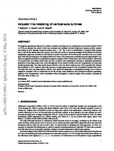
2. Theory: Working Principle of Darrieus-Type Vertical-Axis Wind Turbines (VAWTs) A vertical-axis wind turbine is of Darrieus-type when it is driven by aerodynamic lift [26,42]. The Darrieus turbine consists of two or more aerofoil-shaped blades attached to a rotating vertical shaft. The wind blowing over the aerofoil contours of the blade creates aerodynamic lift and actually pulls the blades along. In this section, general mathematical expressions that describe the aerodynamic models of Darrieus-type VAWTs are presented. Let us consider a curved blade Darrieus-type VAWT as shown in Figure 1. The given aerofoil is characterized by its height 2H, rotor radius R, number of blades Nb = 3 and blade chord c. Consider a given point on any of the blades. r and z are the local radius and height, respectively. When the rotor is subject to an instantaneous incoming wind speed W0 (t ) , it turns at a rotational speed ω(t).

Figure 1. Curved, three-blade, Darrieus-type VAWT. Figure 2 shows the aerodynamic forces and the three velocity vectors acting on Darrieus-type VAWT blade elements at a random position [25,43]. FL and FD are the lift and drag force, respectively. As the blade rotates, the local angle of attack α varies with the relative velocity Wr . The incoming wind speed W0 and the rotational velocity of the blade ω govern the orientation and magnitude of Wr [23,42]. In turn, the forces FL and FD acting on the blade vary. The magnitude and orientation of the lift and drag forces as well as the resultant force vary. The resultant force can be decomposed into a normal force FN and a tangential force FT . The tangential force component then drives the rotation of the wind turbine and produces the torque necessary to generate electricity [24].

Energies 2015, 8

10690

Figure 2. Velocity and force components for a Darrieus-type VAWT (DTVAWT). Elementary normal and tangential forces applied to a blade element are, respectively, given by [44]: c  1 dFN  CN  ρW 2  dz cos δ  2

(1)

c  1 dFT  CT  ρW 2  dz cos δ  2

(2)

H where δ is the pitch angle of the blade, defined as δ  tan 1   ; c is the blade chord (m); and C N  2z  and CT are the normal and tangential force coefficients, respectively, which are given by:

CN  CL cos φ  CD sin φ , CT  CL sin φ  CD cos φ

(3)

where CL and CD are the blade lift and drag coefficients, respectively. These coefficients are related to the blade profile and are obtained from empirical data and made available by the blade manufacturer. CL and CD are experimentally determined and depend on the incidence angle α and the Reynolds Rωc [45]. The lift and drag coefficients are given by the following relations [42]: number Re  W CL 

CD 

Rx ρ  l W 2 2

(4)

Rz

ρ  l W 2 2

(5)

If we assume that the relative dynamic pressure flow q and the blade element area Ae can be 1 expressed as q  ρW 2 and Ae  c  dz , then [46]: 2

Energies 2015, 8

10691 dFN 

CN qAe cos δ

(6)

dFT 

CT qAe cos δ

(7)

The components of the force acting along the x and y Cartesian directions are also called the lift and drag forces. The elementary lift and drag forces are given by [44]: cos θ b   dFL  qc  CN sin θ b  CT  dz cos δ  

(8)

sin θ b   dFD  qc  CN cos θ b  CT  dz cos δ  

(9)

As described in [43,47], the total lift and drag forces, FL and FD , for a single blade can then be calculated by integrating dFL and dFD with respect to the height (  H  z  H ) and the azimuthal revolution ( 0  θ b  2π ). We then obtain: H

FL 

2π

cos θ b c  q  CN sin θ b  CT   2π z  H θ 0  cos δ H

FD 

 dθ b dz 

(10)

2π

sin θ b  c  q  CN cos θ b  CT dθ b dz   2π z  H θ 0  cos δ 

(11)

For a rotor with Nb blades, the average lift and drag forces for the rotor can be defined as: H

FLr 

2π

N bc cos θ b   q  CN sin θ b  CT dθ b dz   2π z  H θ 0  cos δ  H

2π

Nc sin θ b  FDr  b   q  CN cos θ b  CT 2π z  H θ 0  cos δ

 dθ b dz 

(12) (13)

The torque of the Darrieus rotor is produced solely by the tangential component of the applied force [23,43,48]. Thus, from the elementary tangential force of the rotor, we can obtain the elementary torque of the rotor at a given position. For a blade element of length d z / cos δ , we obtain: dTB 

CT qrc dz cos δ

(14)

The torque varies as a function of the azimuthal angle and the rotor height [48]. The total torque can then be obtained by successively integrating the elementary torque with respect to the variables θ and z. For a rotor with Nb blades, we have: xH

TR  N bTB 

cω 2π z xH

2π

qCT r

 cos δ dθ dz b

(15)

0

The average power generated by the rotor shaft is defined as: xH 2π qCT r Ncω P  ωTR  dθ b dz   2π z  xH 0 cos δ

(16)

Energies 2015, 8

10692

The power coefficient of the rotor can then be obtained as: P 81 1 Ncω  Cp  Pmax 64 2π ρV3 RH

xH

2π

qCT r

  cos δ dθ dz b

(17)

z  xH 0

3. Method and Model Construction

Based on the aerodynamic model described in the precedent section, this section is devoted to the presentation of the building process of an equivalent electrical model. Our methodology is based on the complex plane representation of various model subassemblies and an analogy between electrical and mechanical systems. 3.1. The Mechanical-Electrical Analogy Approach The main value of analogies lies in the way in which mathematics unifies these diverse fields of engineering into one subject. Tools developed for solving problems in one field can be used to solve problems in another. This is an important concept because some fields, particularly electrical engineering, have developed rich sets of problem-solving tools that are fully applicable to other engineering fields [49]. There are simple and straightforward analogies between electrical and mechanical systems. Furthermore, analogies between mechanical systems and electrical and fluid systems are effective and are in common use. Two valid techniques of modeling mechanical systems with electrical systems or drawing analogies between the two types of systems can found in the literature, with each method having its own advantages and disadvantages [50–54]. The first technique is intuitive; in this technique, current corresponds to velocity (both are motion), and voltage corresponds to force (both provide a “push”). The second technique is the through/across analogy, which uses voltage as an analogy for velocity and current as an analogy for force. The two schools of thought for modeling mechanical systems with electrical systems are presented in Table 2 [49]. Both are valid. However, the through/across analogy results in a counterintuitive definition of impedance [49,51,52,55]. The analogy for impedance that is universally applied is the one from the intuitive analogy listed in the corresponding section of Table 2. For this reason, the intuitive analogy will be used in the present study.

Energies 2015, 8

10693 Table 2. System analogy used in developing the new model. Topology-Preserving Set (book’s Analogy) Intuitive Analogy Set 

 Topology Change

Intuitive Stretch Description

Trans Mech

“through” variable

(force)

“across” variable

(velocity)

Dissipation

Energy Impedance

(torque)

(current)

Thermal (heat flux)

ν (voltage)

T, θ

ω

Energy

Impedance

Trans Mech

q (flow)

(velocity)

p (pressure)

(force)

Rot Mech ω (angular velocity) (torque)

/

/

or

(one end must be

(one end must be

“grounded”)

“grounded”)

½

½

Standard definition is at right θ

ϕ

½

½ ω

The standard definition of mechanical impedance is the one on the right, based on the intuitive analogy

½

Dissipation

Motion storage

½

(one end must be “grounded”)

Push (force)

ω N/A



Motion

element /

ω or

Description

Dissipative

ω

N/A

/

Across variable storage element

Fluid

ϕ ω /

/

Through-variable storage element

Electrical

ω (angular velocity)



Dissipative element

Rot Mech

(one end usually

“grounded”)

“grounded”)

(not analogous) Θ

Φ

½ ω

Energy

Ω

Impedance

ω

(one end must be

or

or

element

Push (force) storage element

ω

½

Energy Ω

Impedance

Energies 2015, 8

10694

3.2. Wind Flow as an Electric Current Source The analogy between air flow and electrical current is mathematically accurate; the momentum of a section of a gas, also called inertance, is directly analogous to electrical inductance. The compliance of a transmission vessel (hose or pipe) is directly analogous to electrical capacitance [56–59]. In this section, we will model the wind flow across the rotor as an electric current source. Figure 3 shows the top view of a three-blade VAWT and the different velocity components. Considering one of the blades, its shift position xb is characterized by the rotor radius R and the angular position θb . Thus, the complex representation of the blade shift position xb can be written as follows [60–62]: xb  Re jθb

(18)

Figure 3. Top view of a three-blade VAWT showing the velocity components relative to the blade. The linear velocity of the blade W b can be obtained by deriving its position with respect to time. We then have [63]: Wb 

d( xb )  jθ b Re jθb dt

(19)

where θ b =ω is the rotational speed and W0 is the incoming wind and represents wind from any direction. The relative wind seen by the blades at any moment is given by [61,64,65]:    Wr  W0  Wb  W0  jωRe jθb

(20)

As explained in [61], the angle definitions are counter-clockwise; hence, α and φ are negative for the directions of W r and W b (Figure 4). Therefore, if we consider the blade reference frame, the angle of the relative wind is obtained by rotating W r by an angle je jθb , thereby aligning the blade motion

Energies 2015, 8

10695

with the negative real axis. The relative flow velocity for a blade in its own reference frame can then be defined as:





Wrb  Wr  je jθb  W0 je jθb  ωR

(21)

The algebraic expression can be written as follows:

Wrb   ωR  W0 sin θ b   j W0 cos θ b 

(22)

Figure 4. Definition of angles and velocities. The Paraschivoiu model [43] assumes that the direction of the flow does not change. Therefore, the angle of the blade relative to the vertical axis η is taken into consideration when expressing the relative wind velocity seen by the blade. Hence, from Equation (22), the relative wind seen by the blade element, and that corresponding to the streamtube i, can be expressed as follows:

Wrbi   ωRi  W0i sin θ b   j W0i cos θ b  cos ηi

(23)

where η is the angle of the blade relative to the vertical axis and is equal to zero for straight blade VAWTs ( η  0 and cos η  1 ). If the parabola shape of the blade is approximated as: r  z   1   R H

2

(24)

then the angle of the blade relative to the vertical axes can be defined as [43,66]:  H  η  tan 1    tan 1  2  2z  

  1  r R   1

(25)

The angle of the relative wind is the argument of Wrb [9,47]. Because W0 is considered to be real, we can write:   1  cos θ bi cos η i φ i  tan   ωR    i   sin θ bi   W0 i 

where λ 

    tan 1  cos θ bi cos ηi      λ i  sin θ bi   

(26)

ωR is the blade tip speed ratio. W0

Considering the pitch angle δ, the angle of attack α is obtained through summation of the pitch angle and that of the relative wind [23]; specifically:

Energies 2015, 8

10696

α  φδ

(27)

Finally, the wind’s angle of attack relative to a streamtube i can be written as follows:

 cos θ b cos ηi α  tan 1   λ i  sin θ b

   δi 

(28)

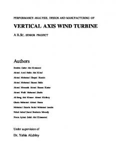
For a given blade element situated at a height z and corresponding to a given streamtube, η and δ are constant. The angle of attack (AoA) will therefore vary with the angle of the relative wind speed, that is, with the rotational angle of the blade. Figure 5 shows the variation of the angle of attack as a function of the rotational angle of the blade for different values of the tip speed ratio λ. The results are in accordance with those obtained in [67] and show that small tip speed ratios lead to large incidence variations during a revolution. 50 Vsp = Vsp = Vsp = Vsp =

40

Wind incident angle in degrees

30

1.5 2 2.5 3

20 10 0 -10 -20 -30 -40 -50

0

100

200

300 400 500 Rotational angle in degrees

600

700

800

Figure 5. Angle of attack as function of the rotational angle.

Additionally, the absolute value of the relative velocity is the modulus of the complex algebraic definition in Equation (22). Therefore, it can be written in accordance with the definition in [68]: 2

 ωR  2 2 Wrb  W0   sin θ b    cos θ b   cos η   W0 

(29)

Broadly speaking, the incident wind at the wind turbine rotor can be written as a complex number:

W rb  Wrb e j (φδ)

(30)

As stated in [56–59], an analogy can be made between the wind flow in a streamtube and an electric current. Equation (30) is similar to the complex expression of a sinusoidal current generator. Moreover, if the incident wind flow is assumed to be an electric current, then the wind relative

Energies 2015, 8

10697

1 ρWrb2 (where q is given in N/m 3 and the fluid density ρ is given in kg/m 3 ), 2 which is the energy acquired by the wind due to its velocity, can be considered as an electric energy source. Referring to our system analogy table, this will be a current source. The wind relative dynamic pressure flow can therefore be written as a complex number:

dynamic pressure flow q 

 

2 2 1 1 1 2 ρ W rb  ρ  Wrb e j (φ  δ)   ρ Wrb e j 2(φ  δ) 2 2 2 2   ωR   1 2 2  sin θ b    cos θ b   cos η   e j 2(φδ) I w  ρV0 2     V0  2   

Iw  q 

(31)

Finally, the instantaneous expression of the current source that represents the relative wind seen by the blade is as follows: iw (t )   cos  ωt  2α   2α

(32)

2     cos θ b cos η  1 2 2 2  ωR  sin θ b    cos θ b   cos η   and α  tan 1  where   ρW0     δ . ψ is the   W0  2 λ i  sin θ b      modulus of the current flow and varies with the rotational angle of the blade. As shown in Figure 6, in the double-multiple multi-streamtube models, the incoming wind speed in the upstream W0u disk is different than that in the downstream disk W0d [69]. Thus, the modulus of the

corresponding current in the downwind disk is slightly lower than that in the upwind disk (    ). We can therefore incorporate this into the current source definition. The new current definition is Equation (33), and the electric current source analogy for wind flow can be represented as shown in Figure 7: d

u  sin  ωt  2α  iw (t )   d   sin  ωt  2α 

for  π / 2  θ  π / 2 for 3π / 2  θ   π / 2

Figure 6. Double-multiple multi-streamtube model.

u

(33)

Energies 2015, 8

10698

Finally, the wind flow in our model is represented as follows:

Figure 7. Wind flow equivalent electrical model. 3.3. Single-Blade Electrical Equivalent Circuit (Normal, Tangential, Lift and Drag Coefficients) The aerodynamic force coefficients acting on a cross-sectional blade element of a Darrieus wind turbine are shown in Figure 8 [70]. The directions of the lift and drag coefficients as well as their normal and tangential components are illustrated.

Figure 8. Aerodynamic coefficients acting on a Darrieus WT blade element [71]. C L and C D denote the lift and drag coefficients, respectively. They are related to the blade profile,

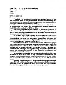
obtained from empirical data, and provided by the blade manufacturer. CL and CD are experimentally determined and depend on the incidence angle α and the Reynolds number [42]. The lift and drag coefficients for 2-D sections are readily available for a wide variety of wing sections at angles of attack up to the point of stall [72]. However, we performed a simulation while varying CL and CD as functions of the rotational angle of the blade for an NACA0012 for the full 360° range of angles. The results are presented in Figure 9 and are in agreement with data in the literature for the corresponding blade profile [17,73–75].

Energies 2015, 8

10699

3.3.1. Writing Normal, Tangential, Lift and Drag Coefficients as Complex Numbers Consider a complex coordinate system defined as shown in Figure 9. 2

Lift and Drag Coefficients

1.5

1

0.5

0

-0.5

-1 Lift Coef Drag Coef -1.5 -200

-150

-100

-50 0 50 Angle of attack in degrees

100

150

200

Figure 9. Lift and drag coefficients variations as a function of the angle of attack for a NACA0012 blade profile.

The vertical axis is assumed to be real, and the horizontal axis is assumed to be imaginary. In this new complex coordinate system, the lift and drag coefficients can be written as complex numbers:

C φ   CL   L      π    φ C C   D   D 2 

(34)

Using the signs of their imaginary components, CL can be regarded as an inductive coefficient with absolute value CL and angle α, and CD can be seen as a capacitive coefficient with absolute value CD π  and angle   φ  . We can therefore write: 2  jφ    CL cos φ  jCL sin φ  CL   CL e     π     π π    j φ      CD   CD e  2    CD cos  φ  2   jCD sin  φ  2       

(35)

 CL   CL cos φ  jCL sin φ        CD   CD sin φ  jCD cos φ 

(36)

which then becomes:

The total or equivalent complex coefficients can be obtained by including the lift and drag coefficients:

Ceq  CL  CD   CL cos φ  jCL sin φ    CD sin φ  jCD cos φ 

(37)

Energies 2015, 8

10700

Grouping real and imaginary components, we obtain: Ceq   CL cos φ  CD sin φ   j  CL sin φ  CD cos φ 

(38)

The tangential force coefficient C T is basically the difference between the tangential components of the lift and drag forces. Similarly, the normal force coefficient C N is the difference between the normal components of the lift and drag forces [25,43,76]. Thus, in the complex plane, C N is real, and C T is imaginary. From Equation (38):

Ceq  CN  jCT

(39)

 CN   CL cos φ  CD sin φ      CT   CL sin φ  CD cos φ 

(40)

where:

The tangential coefficient characterizes the force tangential to the blade. To consider the influence 1 of η on C T , this letter is multiplied by κ  , namely, the coefficient of the blade tilt relative to the cos η

vertical axis; κ  1 for straight-blade VAWTs [43]. Hence, the new definitions of the normal and tangential coefficients that can be applied to any VAWT blade configurations are:  C cos φ  CD sin φ    L  CN   CL cos φ  CD sin φ  cos φ     sin φ    CT   κ  CL sin φ  CD cos φ    CL cos η  CD cos η   

(41)

The lift and drag coefficients become:

sin φ   CL cos φ  jCL   CL  cos η       cos φ   C  D  C sin φ  jC D  D cos η  

(42)

3.3.2. Normal, Tangential, Lift and Drag Impedances The blade is divided into n elements, as shown in Figure 10. Each blade element corresponds to a given streamtube. These blade elements will experience varying flow characteristics because they may have, depending on the design, different radii, angles of relative wind speed, pitch angles, angles relative to the vertical axis, local heights, etc. Our approach is to calculate the characteristics for each blade element. The overall performance of the blade will then be obtained by the discrete addition of the n blade element characteristics along the span of the blade. Each moving body in the air is subjected to a resisting force that tends to oppose this movement. This resistance is a function of the air properties but also depends on the characteristics of the body itself (surface, shape, weight, etc.). Kirchhoff’s first law for air circuits states that the quantity of air leaving a junction must equal the quantity of air entering the junction. Kirchhoff’s second law states that the sum of the pressure drops around any closed path must be equal to zero. Pressure differences and head losses are analogous to

Energies 2015, 8

10701

voltage, electrical current is analogous to volumetric airflow rate and electrical resistance is analogous to airflow resistance [59,77–80]. This approach provides a useful framework when developing an equivalent electrical circuit for a blade.

Figure 10. Discretization of the blade into n elements. To develop our new model, and in accordance with our mechanical-electrical analogy presented in Table 1, the blade resistance will not represent a force; rather, it will represent the capacity of the blade to oppose the wind flow. Thus, the blade element resistance can be defined as [57,81–84]:

Ri  CBi  Ai

(43)

where: -

Ri is the aerodynamic resistance of the blade element; CBi is the equivalent aerodynamic coefficient of the blade; Ai is the cord surface of the blade.

This aerodynamic resistance of the blade element can be decomposed into two components: a horizontal component (in the direction of the flow), which constitutes the drag aerodynamic resistance, and a component perpendicular to the plate, directed upwards, which is called the lift aerodynamic resistance [45]. Based on [57,58,70,85], various impedances of a blade element, because we are using a complex coordinate system, the elementary equivalent impedance of a blade element is obtained by multiplying the corresponding elementary complex coefficient by the elementary surface. Thus, we can write: Z Li  Ai CL  ci  zi  CLi cos φi  jci  zi  CL i

sin φi cos ηi

(44)

From Equation (44), we can write:

ZLi  RLi  jX Li with:

(45)

Energies 2015, 8

10702

 ci  zi  CLi cos φi   RLi        c  z  C sin φi   X Li   i i Li cos η  i  

(46)

where RLi and X Li are the resistive and inductive components of the elementary lift impedance, respectively. Because CLi varies with the angle of attack α , RLi and X Li correspond to a variable

resistor ( RLi  f  αi  ) and a variable inductor ( X Li  f  αi  ), respectively. The equivalent electrical diagram for the lift impedance of a blade element is as shown in Figure 11.

Figure 11. Equivalent electrical diagram for the lift force applied to a blade element.

Identically, the elementary drag impedance is: Z Di  Ai CDi  ci  zi  CD i sin φi  jci  zi  CDi

cos φi cos ηi

(47)

From Equation (47), we can write:

ZDi  RDi  jX Di

(48)

 ci  zi  CDi sin φi   RDi        c  z  C cos φi   X Di   i i Di cos η  i  

(49)

with:

where RDi and X Di are the resistive and inductive components of the elementary drag impedance, respectively. Because CDi varies with the angle of attack α , RDi and X Di will correspond to a variable

resistor ( RDi  f  αi  ) and a variable capacitor ( X Di  f  αi  ), respectively. The equivalent electrical

diagram for the drag impedance of a blade element is as shown in Figure 12.

Figure 12. Equivalent electrical diagram for the drag force applied to a blade element.

3.3.3. Total Impedance and Equivalent Electrical Circuit of a Single Blade From the preceding section, the lift coefficient of the blade produces inductive impedance, and the drag coefficient is responsible for the creation of capacitive impedance. As suggested by the Aynsley resistance approach in [59], the total impedance for a blade element is obtained by adding the elementary lift and drag impedances. We have the following development:

Energies 2015, 8

10703

ZBi  AC i Bi  Ai CLi  CLi  ZLi  ZDi





(50)

Z Bi  Z Li  Z Di

(51)

 sin φi cos φi  Z Bi  ci  zi  CLi cos φi  CDi sin φi   jci  zi  CLi  CDi  cos ηi cos ηi  

(52)

that is:

We can then write:

Finally: Z Bi  ci  zi  CNi  jci  zi 

CTi cos ηi

(53)

From Equation (53), we can write:

Z Bi  Z Ni  ZTi

(54)

where:  C cos φ i  CDi sin φ i  Z Ni   Ri   RLi  RDi   Li     Z   jX   j  X  X    CLi sin φ i  CDi cos φ i i L i D i       Ti  cos ηi cos ηi 

    

(55)

Equations (54) and (55) show that the real component of the total elementary impedance is resistive and is generated by the normal coefficient. In the same vein, the imaginary component of the total elementary impedance is reactive and is produced by the tangential coefficient. This is in accordance with the definitions of the normal and tangential coefficients and forces found in the literature [86]. The total impedance of the entire blade is obtained by the addition of n discrete elementary impedances over the full height of the rotor [87]: n

n

i 1

i 1

Z B   Z Bi    Ri  jX i 

(56)

Specifically: n

n

i 1

i 1

Z B   ci zi CNi  j  ci zi

CTi cos ηi

 sin φi cos φi    ci zi  CL i cos φi  CDi sin φi   j  ci zi  CLi  C Di  cos ηi cos ηi  i 1 i 1  n

n

(57)

We can then write: n  n  Z B    ci zi CLi cos φ i   ci zi CDi sin φ i   i 1  i 1 

If we consider:

n  n sin φ i cos φ i    ci zi CDi j   ci zi CLi  cos ηi i 1 cos ηi   i 1

(58)

Energies 2015, 8

10704

 n   ci zi CLi cos φi  i 1 R  L  n     ci zi CDi sin φi  RD    i 1  XL   n sin φi     ci zi CLi cos ηi  X D   i 1 n  cos φi   ci zi CDi cos ηi  i 1

           

(59)

Z B  RB  jX B  Z N  jZT

(60)

 Z N   RB   RL  RD       ZT   X B   X L  X D 

(61)

We can write:

where:

For a given blade element, the equivalent electrical components are subject to the same wind flow. Thus, the equivalent electrical components of a blade are considered connected in series. Therefore, the electric equivalent circuit for a blade that is subject to a wind flow is as shown in Figure 13.

Figure 13. Electric equivalent circuit for a blade that is subject to a wind flow. 4. Results and Discussion This section presents the obtained equivalent electrical model for a single blade. The simulation results for different elements of the model are also given. The simulations were conducted using data for NACA0012 that can be obtained from different sources in the literature [88–90] with Reynolds numbers ranging from 500,000 to approximately 750,000. Our selection was motivated by the fact that the NACA0012 blade profile is one of the most studied and commonly used as a rotor blade aerofoil section [89]. Finally, the simulation results were assessed using other results that can be found in the literature [91]. 4.1. The Electrical Equivalent Model of a Single Blade The wind flow through the blade (the current flow through the circuit) will produce lift and drag forces (lift and drag voltage) on the one hand and normal and tangential forces (normal and tangential

Energies 2015, 8

10705

voltage) on the other hand. The normal and tangential voltages produced by the blade can be expressed as follows:

 RB2α   VN   Z N I w   RBei 0      2α, 2α          π iπ/2   X 2α      B  VT   Z T I w   X Be  2 

(62)

Following the laws of electrical circuit analyses, the total voltage across a blade can be obtained by the algebraic sum of the lift and drag voltages. We can then write: VB  I w  Z B  I w   Z N  jZ T   VN  VT

(63)

Nevertheless, the torque delivered by the blade is produced only by the tangential component of the force. Therefore, only the tangential voltage will create the power in the corresponding electric circuit. Finally, the electric circuit corresponding to a single blade is obtained. Figure 14 shows the equivalent electric model of a single blade with voltage produce across reactive impedance that stand for blades torque.

Figure 14. The torque produced by the blade reactive impedance. 4.2. Simulations

The simulation characteristics of the rotor were taken from [42] and are presented in Table 3.

Table 3. Blade’s simulation characteristics. Parameter Number of blades Aerofoil section Average blade Reynolds number Aerofoil chord length Rotor tip speed Tip speed ratio Chord-to-radius ratio

Value/spécification 1 NACA0012 40,000 9.14 cm 45.7 cm/s 5 0.15

4.2.1. Variations of Coefficients and Equivalent Electric Components with the Angle of Attack As discussed in Section 4.2, the blade’s lift and drag coefficients vary with the angle of attack of the wind, as shown in Figure 9. These coefficients can then be used to plot the normal and tangential

Energies 2015, 8

10706

coefficients as a function of angle of attack using Equation (3). Furthermore, Figure 5 shows that the angle of attack changes as the blade rotates. Therefore, because the normal and tangential coefficients are obtained using lift and drag, as well as the lift and drag coefficients, the normal and tangential coefficients will vary according the blade position. The variations of the normal and tangential coefficients as functions of the angle of attack can be observed in Figure 15. The obtained results agree with those in [43]. 2

Normal and Tangentiel coefficients

1.5

Normal Coef Tangential Coef

1 0.5 0 -0.5 -1 -1.5 -2 -200

-150

-100

-50 0 50 Angle of attack in degrees

100

150

200

Figure 15. Normal and tangential coefficient variations as functions of the angle of attack.

Using the relations in Equations (59) and (61), we can then find the variations in the various equivalent electrical components according to the angle of attack. The forms of the RB and X B curves follow those of the normal and tangential coefficients. The variations of the values of electric components with the blade angle of attack are plotted on Figures 16 and 17. 1 0.8 0.6

R-Lift R-Drad R-Blade

RL, RD and RB in m2

0.4 0.2 0 -0.2 -0.4 -0.6 -0.8 -1 -200

-150

-100

-50 0 50 Angle of attack in degrees

100

150

200

Figure 16. Lift, drag and normal resistance variations as functions of the angle of attack.

Energies 2015, 8

10707 0.4 X-Lift X-Drag X-Blade

0.3

XL, XD and XB in m2

0.2 0.1 0 -0.1 -0.2 -0.3 -0.4 -200

-150

-100

-50 0 50 Angle of attack in degrees

100

150

200

Figure 17. Reactive element variations as functions of the angle of attack.

4.2.2. Variations of Coefficients and Equivalent Electric Components with the Rotational Angle of the Blade The angle of attack gradually changes as the wind turbine rotor rotates. Figure 6 shows that the angle of attack varies as a function of the rotational angle of the blade; for a tip speed ratio of 1.5, the angle of attack broadly varies between −45° and 45° during a complete rotation of the turbine. Figures 15–17 show that only parts of the various curves, that is, for angles of attack between −50° and 50° are involved in the fluctuations of the respective coefficients and electric elements during a complete rotation of the blade. Figures 18 and 19 simulate the variations of the coefficients as well as the equivalent electrical components according to the blade rotational angle. Our obtained results are consistent with what can be found in the relevant literature in [71]. 1.5

1

m2

0.5

0

-0.5

-1

-1.5

C-Lift C-Drad 0

100

200

300 400 500 Rotational angle in degrees

600

700

800

Figure 18. Lift and drag coefficient variations as functions of rotational angle.

Energies 2015, 8

10708 1.5

C-Nor C-Tang

1

m2

0.5

0

-0.5

-1

-1.5

0

100

200

300 400 500 Rotational angle in degrees

600

700

800

Figure 19. Normal and tangential coefficient variations as functions of rotational angle.

The value of the lift coefficient is almost equal to that drag coefficient, in absolute value, during the rotation of the blade. Meanwhile, the blade’s natural resistance as it moves through the air is nearly equivalent to the surface that opposes the blade weight by generating drag. Indeed, although the lift coefficient values alternate from positive to negative, the drag coefficient always remains positive. The normal and tangential coefficients are non-linear combinations of the lift and drag coefficients. Both are alternative values, and the normal coefficient is much more important. The pressure of air on the surface of the blade varies widely. We can deduce that the surface of the blade that is exposed to the wind pressure varies as the blade rotate. During a complete tour, it is equal to zero for the rotational angles π/2 and 3π/2. The tangential coefficient, responsible for the tangential force and thus of the power produced by the blade, is lower and alternate between positive and negative quantities. We can now plot the variations of various equivalent electrical components with the rotational angle of the blade. The total resistance RB is obtained by algebraic addition of the lift and drag resistances RL and RD. Similarly, the total reactance X B results from the algebraic addition of the lift inductive admittance and drag capacitive admittance. Figures 20 and 21 show that the forms of the RB and X B curves follow those of CN and CT , respectively. This finding is further evidence that the simulation results obtained using the developed model are in agreement with those obtained using existing BEM models.

Energies 2015, 8

10709 0.8

R-Lift R-Drad R-Blade

0.6 0.4

m2

0.2 0 -0.2 -0.4 -0.6 -0.8

0

100

200

300 400 500 Rotational angle in degrees

600

700

800

Figure 20. Lift, drag and normal resistance variations as functions of rotational angle. 0.35

X-Lift X-Drad X-Blade

0.3 0.25

m2

0.2 0.15 0.1 0.05 0 -0.05

0

100

200

300 400 500 Rotational angle in degrees

600

700

800

Figure 21. Lift, drag and normal admittance variations as functions of rotational angle.

4.2.3. Cross Validation and Comparative Analysis Finally, to perform the cross validation simulation, the results of the normal and tangential forces obtained with equivalent electric model (EEM) were compared with those obtained using DMSTM. The simulation results of the normal and tangential forces using the EEM model and DMSTM of DTVAWTs are superimposed. The obtained results are shown in Figures 22 and 23.

Energies 2015, 8

10710 300

Fn-eem Fn-dmstm

200

m2

100

0

-100

-200

-300

0

100

200

300 400 500 Rotational angle in degrees

600

700

800

Figure 22. Cross validation of normal force variations as functions of rotational angle. 30

Ft-eem Ft-dmstm

25 20 15

m2

10 5 0 -5 -10 -15 -20

0

100

200

300 400 500 Rotational angle in degrees

600

700

800

Figure 23. Cross validation of tangential force variations as functions of rotational angle.

Figures 22 and 23 show that EEM produces satisfactory results as these results are in agreement with the results obtained in [43,92] for a single blade. Indeed, even though a slight distortion between the EEM and DMSTM normal forces can be observed on Figure 22. Figure 23 clearly shows that the EEM and DMSTM tangential forces strongly overlap.

Energies 2015, 8

10711

5. Conclusions

A new approach for modeling Darrieus-type VAWT rotors using the electric-mechanic analogy was presented. This paper provides a proof-of-concept demonstration of the approach and attests to the feasibility of such a model through both step-by-step demonstrations of the theoretical and practical concepts that underpin the new model and simulations and cross validation of a single blade model. The obtained simulation results tie in with the findings of the Paraschivoiu double-multiple streamtube model found in the literature. An equivalent electrical model for Darrieus-type VAWTs was proven to be viable. We intend in our future work to finalize the model building process and address the electrical modeling of the blades’ mechanical coupling to the shaft to generate an EEM for the full three-blade DTVAWT rotor. A comparative study of the results of the new model and those of existing models will then conducted. The model that will emerge from this new approach is likely to be more appropriate for the design, performance prediction and optimization of Darrieus rotors. Mechanical fault diagnosis and prognosis is also an important aspect because the model could be used to simulate the rotor’s behavior in the case of mechanical faults in one or more of the blades as well as in rotor-shaft coupling elements. The model will also enable the simulation of turbine operation in the case of mechanical faults in one or more elements of the rotor. Although further work must be conducted to build an EEM for the entire VAWT turbine, the findings of this study are encouraging and have practical applications for the determination and understanding of the aerodynamic factors that influence the performance of Darrieus-type VAWTs under different operating conditions. In future works, the results of the EEM for DTVAWTs will be considered for extension to other types of wind turbines, including horizontal axis and Savonious types. Additionally, the EEM of rotors may be used to study the influence of wind flow turbulence on turbine vibrations. Transitional (starting) and permanent sate functioning of VAWTs may also be examined. We will also use the model to simulate the behavior of a Darrieus WT in the case of a structural break in one or more blades. Finally, as a long-term goal, the EEM of the rotor will be linked to existing models of other electrical and mechanical parts to obtain a global model of a Darrieus WECS. Acknowledgments

The authors would like to thank the Natural Science and Engineering Research Council of Canada (NSERC) for financially supporting this research. Authors’ gratefulness also goes to the editor and four anonymous reviewers for their valuable comments and suggestions that appreciably improved the quality of this paper. Author Contributions

Pierre Tchakoua is the main author of this work. This paper provides a further elaboration on some of the results from his Ph.D. dissertation. René Wamkeue and Mohand Ouhrouche supervised the project and thus supported Pierre Tchakoua’s research in terms of both scientific and technical expertise. Tommy Andy Tameghe and Gabriel Ekemb participated in results analysis and interpretation.

Energies 2015, 8

10712

The manuscript is written by Pierre Tchakoua and revised and commented by René Wamkeue and Mohand Ouhrouche. Conflicts of Interest

The authors declare no conflict of interest. References

1. 2. 3. 4.

5.

6.

7.

8. 9.

10. 11. 12.

13.

Scheurich, F.; Brown, R.E. Modelling the aerodynamics of vertical-axis wind turbines in unsteady wind conditions. Wind Energy 2013, 16, 91–107. Howell, R.; Qin, N.; Edwards, J.; Durrani, N. Wind tunnel and numerical study of a small vertical axis wind turbine. Renew. Energy 2010, 35, 412–422. Eriksson, S.; Bernhoff, H.; Leijon, M. Evaluation of different turbine concepts for wind power. Renew. Sustain. Energy Rev. 2008, 12, 1419–1434. Castelli, M.R.; Grandi, G.; Benini, E. Numerical analysis of the performance of the DU91-W2-250 airfoil for straight-bladed vertical-axis wind turbine application. World Acad. Sci. Eng. Technol. 2012, 6, 742–747. Ferreira, C.S.; Bussel, G.; Kuik, G.V. 2D CFD Simulation of Dynamic Stall on a Vertical Axis Wind Turbine: Verification and Validation with PIV Measurements. In Proceedings of the 45th AIAA Aerospace Sciences Meeting and Exhibit, Reno, NV, USA, 8–11 January 2007; pp. 1–11. Tjiu, W.; Marnoto, T.; Mat, S.; Ruslan, M.H.; Sopian, K. Darrieus vertical axis wind turbine for power generation I: Assessment of Darrieus VAWT configurations. Renew. Energy 2015, 75, 50–67. Tjiu, W.; Marnoto, T.; Mat, S.; Ruslan, M.H.; Sopian, K. Darrieus vertical axis wind turbine for power generation II: Challenges in HAWT and the opportunity of multi-megawatt Darrieus VAWT development. Renew. Energy 2015, 75, 560–571. Bianchini, A.; Ferrara, G.; Ferrari, L. Design guidelines for H-Darrieus wind turbines: Optimization of the annual energy yield. Energy Convers. Manag. 2015, 89, 690–707. Dixon, K.R. The Near Wake Structure of a Vertical Axis Wind Turbine Including the Development of a 3D Unsteady Free-Wake Panel Method for VAWTs. Master’s Thesis, Delft University of Technology, Delft, The Netherlands, 2008. Carrigan, T.J.; Dennis, B.H.; Han, Z.X.; Wang, B.P. Aerodynamic shape optimization of a vertical-axis wind turbine using differential evolution. ISRN Renew. Energy 2011, 2012, 1–16. Lanzafame, R.; Mauro, S.; Messina, M. 2D CFD modeling of H-Darrieus wind turbines using a transition turbulence model. Energy Procedia 2014, 45, 131–140. Tchakoua, P.; Wamkeue, R.; Tameghe, T.A.; Ekemb, G. A Review of Concepts and Methods for Wind Turbines Condition Monitoring. In Proceedings of the 2013 World Congress on Computer and Information Technology (WCCIT), Sousse, Tunisia, 22–24 June 2013; pp. 1–9. Tchakoua, P.; Wamkeue, R.; Ouhrouche, M.; Slaoui-Hasnaoui, F.; Tameghe, T.; Ekemb, G. Wind turbine condition monitoring: State-of-the-art review, new trends, and future challenges. Energies 2014, 7, 2595–2630.

Energies 2015, 8

10713

14. Tchakoua, P.; Wamkeue, R.; Slaoui-Hasnaoui, F.; Tameghe, T.A.; Ekemb, G. New Trends and Future Challenges for Wind Turbines Condition Monitoring. In Proceeding of the 2013 International Conference on Control, Automation and Information Sciences (ICCAIS), Nha Trang, Vietnam, 25–28 November 2013; pp. 238–245. 15. Chen, Y.; Lian, Y. Numerical investigation of vortex dynamics in an H-rotor vertical axis wind turbine. Eng. Appl. Comp. Fluid Mech. 2015, 9, 21–32. 16. Jin, X.; Zhao, G.; Gao, K.; Ju, W. Darrieus vertical axis wind turbine: Basic research methods. Renew. Sustain. Energy Rev. 2015, 42, 212–225. 17. Paraschivoiu, I. Double-multiple streamtube model for Darrieus in turbines. Wind Turbine Dyn. 1981, 1, 19–25. 18. Mohamed, M.H. Performance investigation of H-rotor Darrieus turbine with new airfoil shapes. Energy 2012, 47, 522–530. 19. Masson, C.; Leclerc, C.; Paraschivoiu, I. Appropriate dynamic-stall models for performance predictions of VAWTs with NLF blades. Int. J. Rotat. Mach. 1998, 4, 129–139. 20. Dyachuk, E.; Goude, A. Simulating dynamic stall effects for vertical Axis wind turbines applying a double multiple Streamtube model. Energies 2015, 8, 1353–1372. 21. Dai, Y.M.; Gardiner, N.; Sutton, R.; Dyson, P.K. Hydrodynamic analysis models for the design of Darrieus-type vertical-axis marine current turbines. Proc. Inst. Mech. Eng. M J. Eng. Marit. Environ. 2011, 225, 295–307. 22. Hall, T.J. Numerical Simulation of a Cross Flow Marine Hydrokinetic Turbine. Ph.D. Thesis, University of Washington, Seattle, WA, USA, 2012. 23. Islam, M.; Ting, D.S.K.; Fartaj, A. Aerodynamic models for Darrieus-type straight-bladed vertical axis wind turbines. Renew. Sustain. Energy Rev. 2008, 12, 1087–1109. 24. Beri, H.; Yao, Y. Double multiple Streamtube model and numerical analysis of vertical axis wind turbine. Energy Power Eng. 2011, 3, 262–270. 25. Zhang, L.X.; Liang, Y.B.; Liu, X.H.; Jiao, Q.F.; Guo, J. Aerodynamic performance prediction of straight-bladed vertical axis wind turbine based on CFD. Adv. Mech. Eng. 2015, 5, doi:10.1155/2013/905379. 26. Bhutta, M.M.A.; Hayat, N.; Farooq, A.U.; Ali, Z.; Jamil, S.R.; Hussain, Z. Vertical axis wind turbine—A review of various configurations and design techniques. Renew. Sustain. Energy Rev. 2012, 16, 1926–1939. 27. Edwards, J. The Influence of Aerodynamic Stall on the Performance of Vertical Axis Wind Turbines. Ph.D. Thesis, University of Sheffield, Sheffield, UK, 2012. 28. Alaimo, A.; Esposito, A.; Messineo, A.; Orlando, C.; Tumino, D. 3D CFD analysis of a vertical axis wind turbine. Energies 2015, 8, 3013–3033. 29. Verkinderen, E.; Imam, B. A simplified dynamic model for mast design of H-Darrieus vertical axis wind turbines (VAWTs). Eng. Struct. 2015, 100, 564–576. 30. Chowdhury, A.M.; Akimoto, H.; Hara, Y. Comparative CFD analysis of vertical axis wind turbine in upright and tilted configuration. Renew. Energy 2016, 85, 327–337. 31. Tilmans, H.A.C. Equivalent circuit representation of electromechanical transducers: I. Lumped-parameter systems. J. Micromech. Microeng. 1996, 6, 157–176.

Energies 2015, 8

10714

32. Mason, W. An electromechanical representation of a piezoelectric crystal used as a transducer. Proc. Inst. Radio Eng. 1935, 23, 1252–1263. 33. Tilmans, H.A.C. Equivalent circuit representation of electromechanical transducers: II. Distributed-parameter systems. J. Micromech. Microeng. 1997, 7, 285–309. 34. Barakati, S.M. Modeling and Controller Design of a Wind Energy Conversion System Including a Matrix Converter. Ph.D. Thesis, University of Waterloo, Waterloo, ON, Canada, 2008. 35. Kim, H.; Kim, S.; Ko, H. Modeling and control of PMSG-based variable-speed wind turbine. Electr. Power Syst. Res. 2010, 80, 46–52. 36. Borowy, B.S.; Salameh, Z.M. Dynamic response of a stand-alone wind energy conversion system with battery energy storage to a wind gust. IEEE Trans. Energy Conver. 1997, 12, 73–78. 37. Delarue, P.; Bouscayrol, A.; Tounzi, A.; Guillaud, X.; Lancigu, G. Modelling, control and simulation of an overall wind energy conversion system. Renew. Energy 2003, 28, 1169–1185. 38. Slootweg, J.G.; de Haan, S.W.H.; Polinder, H.; Kling, W.L. General model for representing variable speed wind turbines in power system dynamics simulations. IEEE Trans. Power Syst. 2003, 18, 144–151. 39. Junyent-Ferré, A.; Gomis-Bellmunt, O.; Sumper, A.; Sala, M.; Mata, M. Modeling and control of the doubly fed induction generator wind turbine. Simul. Model. Pract. Theory 2010, 18, 1365–1381. 40. Bolik, S.M. Modelling and Analysis of Variable Speed Wind Turbines with Induction Generator during Grid Fault. Ph.D. Thesis, Aalborg University: Aalborg, Danmark, 2004. 41. Perdana, A. Dynamic Models of Wind Turbines; Chalmers University of Technology: Göteborg, Sweden, 2008. 42. Scheurich, F.; Fletcher, T.M.; Brown, R.E. Simulating the aerodynamic performance and wake dynamics of a vertical-axis wind turbine. Wind Energy 2011, 14, 159–177. 43. Paraschivoiu, I. Wind Turbine Design: With Emphasis on Darrieus Concept; Polytechnic International Press: Montréal, QC, Canada, 2002. 44. Claessens, M. The Design and Testing of Airfoils for Application in Small Vertical Axis Wind Turbines. Master’s Thesis, Delft University of Technology, Delft, The Netherlands, 2006. 45. Ajedegba, J.O.; Naterer, G.; Rosen, M.; Tsang, E. Effects of Blade Configurations on Flow Distribution and Power Output of a Zephyr Vertical Axis Wind Turbine. In Proceedings of the 3rd IASME/WSEAS International Conference on Energy & Environment, Stevens Point, WI, USA, 23 February 2008; pp. 480–486. 46. Camporeale, S.M.; Magi, V. Streamtube model for analysis of vertical axis variable pitch turbine for marine currents energy conversion. Energy Convers. Manag. 2000, 41, 1811–1827. 47. Scheurich, F. Modelling the Aerodynamics of Vertical-Axis Wind Turbines. Ph.D. Thesis, University of Glasgow, Glasgow, UK, 2011. 48. Chandramouli, S.; Premsai, T.; Prithviraj, P.; Mugundhan, V.; Velamati, R.K. Numerical analysis of effect of pitch angle on a small scale vertical axis wind turbine. Int. J. Renew. Energy Res. 2014, 4, 929–935. 49. Lewis, J.W. Modeling Engineering Systems: PC-Based Techniques and Design Tools; LLH Technology Publishing: Eagle Rock, VA, USA, 1994. 50. Hogan, N.; Breedveld, P. The physical basis of analogies in network models of physical system dynamics. Simul. Ser. 1999, 31, 96–104.

Energies 2015, 8

10715

51. Firestone, F.A. A new analogy between mechanical and electrical systems. J. Acoust. Soc. Am. 1933, 4, 249–267. 52. Olson, H.F. Dynamical Analogies; D. Van Nostrand Company, Inc.: Princeton, NJ, USA, 1959. 53. Firestone, F.A. The mobility method of computing the vibration of linear mechanical and acoustical systems: Mechanical-electrical analogies. J. Appl. Phys. 1938, 9, 373–387. 54. Calvo, J.A.; Alvarez-Caldas, C.; San, J.L. Analysis of Dynamic Systems Using Bond. Graph. Method through SIMULINK; INTECH Open Access Publisher: Rijeka, Croatia, 2011. 55. Bishop, R.H. Mechatronics: An Introduction; CRC Press: Boca Raton, FL, USA, 2005. 56. Van Gilder, J.W.; Schmidt, R.R. Airflow Uniformity through Perforated Tiles in a Raised-Floor Data Center. In Proceedings of the ASME 2005 Pacific Rim Technical Conference and Exhibition on Integration and Packaging of MEMS, NEMS, and Electronic Systems collocated with the ASME 2005 Heat Transfer Summer Conference, San Francisco, CA, USA, 17–22 July 2005; pp. 493–501. 57. Pugh, L.G.C.E. The influence of wind resistance in running and walking and the mechanical efficiency of work against horizontal or vertical forces. J. Physiol. 1971, 213, 255–276. 58. Herrmann, F.; Schmid, G.B. Analogy between mechanics and electricity. Eur. J. Phys. 1985, 6, 16–21. 59. Aynsley, R.M. A resistance approach to analysis of natural ventilation airflow networks. J. Wind Eng. Ind. Aerodyn. 1997, 67, 711–719. 60. Deglaire, P. Analytical Aerodynamic Simulation Tools for Vertical Axis Wind Turbines. Ph.D. Thesis, Acta Universitatis Upsaliensis, Uppsala, Sweden, 2010. 61. Goude, A. Fluid Mechanics of Vertical Axis Turbines: Simulations and Model Development. Ph.D. Thesis, Uppsala University, Uppsala, Sweden, 2012. 62. Dyachuk, E.; Goude, A.; Bernhoff, H. Dynamic stall modeling for the conditions of vertical Axis wind turbines. AIAA J. 2014, 52, 72–81. 63. Wilson, R.E.; Walker, S.N.; Lissaman, P.B.S. Aerodynamics of the Darrieus rotor. J. Aircr. 1976, 13, 1023–1024. 64. Goude, A.; Lundin, S.; Leijon, M. A Parameter Study of the Influence of Struts on the Performance of a Vertical-Axis Marine Current Turbine. In Proceedings of the 8th European Wave and Tidal Energy Conference (EWTEC09), Uppsala, Sweden, 7–10 September 2009; pp. 477–483. 65. Wekesa, D.W.; Wang, C.; Wei, Y.; Danao, A.M. Influence of operating conditions on unsteady wind performance of vertical axis wind turbines operating within a fluctuating free-stream: A numerical study. J. Wind Eng. Ind. Aerodyn. 2014, 135, 76–89. 66. Shires, A. Development and evaluation of an aerodynamic model for a novel vertical axis wind turbine concept. Energies 2013, 6, 2501–2520. 67. Antheaume, S.; Maître, T.; Achard, J. Hydraulic Darrieus turbines efficiency for free fluid flow conditions versus power farms conditions. Renew. Energy 2008, 33, 2186–2198. 68. Butbul, J.; MacPhee, D.; Beyene, A. The impact of inertial forces on morphing wind turbine blade in vertical axis configuration. Energy Convers. Manag. 2015, 91, 54–62. 69. Jamati, F. Étude Numérique d’une Éolienne Hybride Asynchrone. Ph.D. Thesis, Polytechnique Montréal, Montréal, QC, Canada, 2011.

Energies 2015, 8

10716

70. Batista, N.C.; Melìcio, R.; Matias, J.C.O.; Catalao, J.P.S. Self-Start Performance Evaluation in Darrieus-Type Vertical Axis Wind Turbines: Methodology and Computational Tool Applied to Symmetrical Airfoils. In Proceedings of the International Conference on Renewable Energies and Power Quality (ICREPQ’11), Las Palmas de Gran Canaria, Spain, 13–15 April 2011. 71. Patel, M.V.; Chaudhari, M.H. Performance Prediction of H-Type Darrieus Turbine by Single Stream Tube Model for Hydro Dynamic Application. Int. J. Eng. Res. Technol. 2013, 2. 72. Abbott, I.H.; Von Doenhoff, A.E. Theory of Wing Sections, Including a Summary of Airfoil Data; Courier Corporation: North Chelmsford, MA, USA, 1959. 73. Evans, J.; Nahon, M. Dynamics modeling and performance evaluation of an autonomous underwater vehicle. Ocean Eng. 2004, 31, 1835–1858. 74. Wu, J.; Lu, X.; Denny, A.G.; Fan, M.; Wu, J. Post-stall flow control on an airfoil by local unsteady forcing. J. Fluid Mech. 1998, 371, 21–58. 75. Castelli, M.R.; Fedrigo, A.; Benini, E. Effect of dynamic stall, finite aspect ratio and streamtube expansion on VAWT performance prediction using the BE-M model. Int. J. Eng. Phys. Sci. 2012, 6, 237–249. 76. Tala, H.; Patel, H.; Sapra, R.R.; Gharte, J.R. Simulations of small scale straight blade Darrieus wind turbine using latest CAE techniques to get optimum power output. Int. J. Adv. Found. Res. Sci. Eng. 2014, 1, 37–53. 77. Hartman, H.L.; Mutmansky, J.M.; Ramani, R.V.; Wang, Y. Mine Ventilation and Air Conditioning; John Wiley & Sons: San Francisco, CA, USA, 2012. 78. Aynsley, R. Indoor wind speed coefficients for estimating summer comfort. Int. J. Vent. 2006, 5, 3–12. 79. McPherson, M.J. Ventilation network analysis. In Subsurface Ventilation and Environmental Engineering; Springer: Amsterdam, The Netherlands, 1993; pp. 209–240. 80. Acuña, E.I.; Lowndes, I.S. A review of primary mine ventilation system optimization. Interfaces 2014, 44, 163–175. 81. Sheldon, J.C.; Burrows, F.M. The dispersal effectiveness of the achene—Pappus units of selected Compositae in steady winds with convection. New Phytol. 1973, 72, 665–675. 82. Toussaint, H.M.; de Groot, G.; Savelberg, H.H.; Vervoorn, K.; Hollander, A.P.; van Ingen Schenau, G.J. Active drag related to velocity in male and female swimmers. J. Biomech. 1988, 21, 435–438. 83. Cresswell, L.G. The relation of oxygen intake and speed in competition cycling and comparative observations on the bicycle ergometer. J. Physiol. 1974, 241, 795–808. 84. Martin, J.C.; Milliken, D.L.; Cobb, J.E.; McFadden, K.L.; Coggan, A.R. Validation of a mathematical model for road cycling power. J. Appl. Biomech. 1998, 14, 276–291. 85. Kiyoto, H.; Tosha, K. Effect of Peened Surface Characteristics on Flow Resistance. In Proceedings of the 10th International Conference on Shot Peening, Tokyo, Japan, 15–18 September 2008; pp. 535–540. 86. Crawford, C. Advanced Engineering Models for Wind Turbines with Application to the Design of a Coning Rotor Concept. Ph.D. Thesis, University of Cambridge, Cambridge, UK, 2007.

Energies 2015, 8

10717

87. Mohammadi-Amin, M.; Ghadiri, B.; Abdalla, M.M.; Haddadpour, H.; de Breuker, R. Continuous-time state-space unsteady aerodynamic modeling based on boundary element method. Eng. Anal. Bound. Elem. 2012, 36, 789–798. 88. Sheldahl, R.E.; Klimas, P.C. Aerodynamic Characteristics of Seven Symmetrical Airfoil Sections through 180-Degree Angle of attack for Use in Aerodynamic Analysis of Vertical Axis Wind Turbines; Technical Report for Sandia National Laboratories: Albuquerque, NM, USA, 1981. 89. Critzos, C.C.; Heyson, H.H.; Boswinkle, R.W. Aerodynamic Characteristics of NACA 0012 Airfoil Section at Angles of Attack from 0 Degree to 180 Degree; Technical Report for National Advisory Committee for Aeronautics, Langley Aeronautical Lab: Langley Field, VA, USA, 1955. 90. Miley, S.J. A Catalog of Low Reynolds Number Airfoil Data for Wind Turbine Applications; Technical Rockwell International Corp: Golden, CO, USA, 1982. 91. Timmer, W.A. Aerodynamic Characteristics of Wind Turbine Blade Airfoils at High Angles-of-Attack. In Proceedings of the 3rd EWEA Conference-Torque 2010: The Science of making Torque from Wind, Heraklion, Greece, 28–30 June 2010. 92. Rathi, D. Performance Prediction and Dynamic Model Analysis of Vertical Axis Wind Turbine Blades with Aerodynamically Varied Blade Pitch. Master’s Thesis, NC State University, Raleigh, NC, USA, 2012. © 2015 by the authors; licensee MDPI, Basel, Switzerland. This article is an open access article distributed under the terms and conditions of the Creative Commons Attribution license (http://creativecommons.org/licenses/by/4.0/).