A New Approach to Parallel Preconditioning with Sparse Approximate ...

A New Approach to Parallel Preconditioning with Sparse Approximate Inverses Thomas Huckle and Marcus Grote September 20, 1994 Abstract

A new parallel preconditioner is presented for the solution of large, sparse, nonsymmetric linear systems of equations. A sparse approximate inverse is computed explicitly, and then applied as a preconditioner to an iterative method. The computation of the preconditioner is inherently parallel, and its application only requires a matrix-vector product. The sparsity pattern of the approximate inverse is not imposed a priori but captured automatically. This keeps the amount of work and the number of nonzero entries in the preconditioner to a minimum. Rigorous bounds on the clustering of the eigenvalues and the singular values are derived for the preconditioned system, and the proximity of the approximate to the true inverse is estimated. An extensive set of test problems from scienti c and industrial applications provides convincing evidence of the eectiveness of this new approach.

1 Introduction We consider the linear system of equations Ax = b; x; b 2 IRn : (1) Here A is a large, sparse, and nonsymmetric matrix. Due to the size of A, direct solvers become prohibitively expensive because of the amount of work and storage required. As an alternative we consider iterative methods such as gmres, bcg, bi-cgstab, and cg applied to the normal equations 1

[4]. Given the initial guess x0, these algorithms compute iteratively new approximations xk to the true solution x = A?1b. The iterate xm is accepted as a solution if the residual rm = b?Axm satis es krmk=kbk  tol. In general, the convergence is not guaranteed, or may be extremely slow. Hence, the original problem (1) must be transformed into a more tractable form. To do so, we consider a preconditioning matrix M , and apply the iterative solver either to the right or to the left preconditioned system

AMy = b ; x = My ; or MAx = Mb :

(2)

Therefore, M should be chosen such that AM is a good approximation of the identity. As the ultimate goal is to reduce the total execution time, both the computation of M and the matrix-vector product with M should be evaluated in parallel. Since the matrix-vector product must be performed at each iteration, the amounts of ll-in of A and M should be similar. The most successful preconditioning methods in terms of reducing the number of iterations, such as incomplete LU factorizations or SSOR, are notoriously dicult to implement on a parallel architecture, especially for unstructured matrices. Indeed, the application of the preconditioner in the iteration phase requires the solution of triangular systems at each step, which is dicult to parallelize because of the recursive nature of the computation (see [1], section 4.4.4). Our aim is to nd an inherently parallel preconditioner, which retains the convergence properties of incomplete LU . A natural way to achieve parallelism is to compute an approximate inverse M of A, such that AM ' I in some sense. The evaluation of My is then easy to parallelize, and will be cheap if M is sparse. Although such a sparse approximate inverse does not always exist, it often occurs in applications that most entries in A?1 are very small [3]. For instance, if the problem results from the discretization of a partial dierential equation, it is generally meaningful to look for a sparse approximate inverse. Polynomial preconditioners with M = p (A) are inherently parallel, but do not lead to as much improvement in the convergence as incomplete LU (see [1], section 3.5). We propose a dierent approach, and try to minimize kAM ? I k. Yet we cannot con ne the whole spectrum of AM to the vicinity of 1, or else we would be minimizing the `1 or `2 norm which would be too expensive, since M = 0 is a better solution as long as kAM ? I k > 1. To ensure 2

fast convergence at a reasonable cost, we need to cluster most eigenvalues and singular values about 1, but give a few outliers additional freedom. We achieve this by minimizing kAM ? I k in the Frobenius norm. Moreover, this choice naturally leads to inherent parallelism, because the columns mk of M can be computed independently of one another. Indeed, since n X kAM ? I k2F = k(AM ? I )ek k22 ; (3) k=1

the solution of (3) separates into n independent least squares problems min m kAmk ? ek k2 ; k = 1; : : : ; n ; k

(4)

where ek = (0; :::; 0; 1; 0; :::; 0)T . Thus, we can solve (4) in parallel and obtain an explicit approximate inverse M of A. If M is sparse, (4) reduces to n small least squares problems, which can be solved very quickly [7],[11]. The diculty lies in determining a good sparsity structure of the approximate inverse, or else the solution of (4) will not yield an eective preconditioner. Thus, we look for a method that captures the sparsity pattern of the main entries of A?1 automatically. We start with a given sparsity pattern, such as diagonal, and augment M progressively until the `2 norm of the residual is small enough or a maximal amount of ll-in in M has been reached. Similar approaches based on minimizing (4) can be found in the literature. Yeremin et al. compute a factorized sparse approximate inverse [9], [10], [11], but they only consider xed sparsity patterns. Simon and Grote solve (4) explicitly, but only allow for a banded sparsity pattern in M [7],[8]. In [6] the sparsity of the approximate inverse is selected dynamically, but the criteria for choosing new elements are oriented towards reducing the `1 norm. A recent approach by Chow and Saad [2] uses an iterative method to compute an approximate solution of (4). Although their method generates new entries in M automatically at each iteration, they must apply a drop strategy to remove the excessive ll-in appearing in M . In section 2 we introduce the SPAI algorithm to compute a sparse approximate inverse. In section 3 we derive theoretical properties of the spectrum of the preconditioned system. In sections 4 and 5 we present a wide range of numerical experiments using large test matrices from engineering and scienti c applications. 3

2 The Computation of the Sparse Approximate Inverse We shall rst show how to compute a sparse approximate M for a given sparsity structure. The matrix M is the solution of the minimization problem (4). Since the columns of M are independent of one another, we only need to present the algorithm for one of them, and we denote it by mk . Now let J be the set of indices j such that mk (j ) 6= 0 . We denote the reduced vector of unknowns mk (J ) by m^ k . Next, let I be the set of indices i such that A(i; J ) is not identically zero. This enables us to eliminate all zero rows in the submatrix A(:; J ) . We denote the resulting submatrix A(I ; J ) by A^ . Similarly, we de ne e^k = ek (I ) . If we now set n1 = jIj and n2 = jJ j, we see that solving (4) for mk is equivalent to solving min kA^m^ k ? e^k k2 (5) m^ k

for m^k . The n1  n2 least squares problem (5) is extremely small because A and M are very sparse matrices. If A is nonsingular, the submatrix A^ must have full rank. Thus, the QR-decomposition of A^ is R ^ A=Q 0 ; (6) where R is a nonsingular upper triangular n2  n2 matrix. If we let c^ = QT e^k , the solution of (5) is m^ k = R?1 c^ (1 : n2) : (7) We solve (7) for each k = 1; : : : ; n and set mk (J ) = m^ k . This yields an approximate inverse M , which minimizes kAM ? I kF for the given sparsity structure. Our aim is now to improve upon M by augmenting its sparsity structure to obtain a more eective preconditioner. To do so, we must reduce the current error kAM ? I kF , that is reduce kAmk ? ek k2 for each k = 1; : : :; n . We recall that m^ k is the optimal solution of the least squares problem (4), and denote its residual by

r = A(:; J ) m^ k ? ek : 4

(8)

If r were zero, mk would exactly be the k-th column of A?1, and could not be improved upon. We now assume that r 6= 0 and demonstrate how to augment the set of indices J to reduce krk2 . Since A and mk are sparse, most components of r are zero, and we denote by L the remaining set of indices l, for which r(l) 6= 0 . Typically L is equal to I , since r^ does not have exact zero entries in nite precision. But if I does not contain k, it must be included in L since r(k) is then equal to 1. To every l 2 L corresponds an index set Nl, which consists of the indices of the nonzero elements of A(l; :) that are not in J yet. The potential new candidates, which might be added to J , are contained in [ J~ = Nl : (9) l2L

We must now select new indices j that will lead to the most pro table reduction in krk2. To do so in a cheap but eective way, we consider for each j 2 J~ the one dimensional minimization problem min kr + j Aej k2 :

(10)

T j = ? krAeAekj2 :

(11)

j 2IR

The solution of (10) is

j

2

For each j we compute the `2 norm j of the new residual r + j Aej with j given by (11): T 2 2j = krk22 ? (kr AeAekj 2) : (12) j

2

There is at least one index j 2 J~ such that 6= 0, which will lead to a smaller residual in (12). Otherwise 0 = r(L)T A(L; J~) = r(L)T A(L; J [ J~) ; (13)

rT Aej

which would imply that r(L) is zero, since A(L; :) has full rank. We note that J [ J~ contains the column indices of all nonzero elements of A(L; :), and that J \ J~ = ; . We reduce J~ to the set of the most pro table indices j with smallest j , and add it to J . Using the augmented set of indices J , we solve the sparse least squares problem (4) again. This yields a better approximation mk of the k-th column of A?1. We repeat this process for 5

each k = 1; : : :; n; until the residual satis es a prescribed tolerance or a maximum amount of ll-in has been reached in mk . The numerical study in section 4 shows that this iterative procedure captures the main entries in A?1 extremely well. Every time we augment the set of nonzero entries in mk , we solve the least squares problem exactly. We shall now demonstrate how one can easily update the QR decomposition, and greatly reduce the amount of work. We recall that J is the current set and that J~ is the set of new indices that will be added to mk . We denote by I~ the new corresponding rows that contain the nonzero rows of A(:; J [ J~), and by n~ 1 and n~ 2 the corresponding sizes of I~ and J~. Thus, we need to replace the submatrix A^ by the larger submatrix A(I [ I~; J [ J~). To do so, we use the known QR decomposition of A^ to update the QR decomposition of the augmented matrix A(I [ I~; J [ J~):  A^ A(I ; J~)  ~ ~ A(I [ I ; J [ J ) = 0 A(I~; J~) = (14) 0 1 Q  R QT1 A(I ; J~) Q R B  B C 1 T ~ = (15) In~1 @ 00 QA2 A(I~(;IJ;~J) ) A = In~1 0 B2 : This requires only the computation of the QR decomposition of B2 . We note that A(I~; J ) = 0, because I already contains the indices of all nonzero entries present in columns J . We let  R~  ~ B2 = Q 0 ; (16) where B2 is a n~ 1 + n1 ? n2  n~ 2 matrix. Using (16) we rewrite (15) as 0 1 Q  I  B R B1 C n2 ~ A(I [ I~; J [ J~) = (17) In~1 Q~ @ 00 R0 A :

This enables us to add new indices to J and solve the least squares problem for the optimal solution without recomputing the full QR decomposition at each step. If we do not stop the process, the algorithm will compute the k-th column of A?1. In practice, however, we stop the process once the prescribed tolerance is met or a maximal amount of ll-in has been reached. We now 6

present the full SPAI algorithm, where SPAI stands for SParse Approximate Inverse:

The SPAI Algorithm:

For every column mk of M : (a) Choose an initial sparsity J . (b) Compute the row indices I of the corresponding nonzero entries and the QR decomposition (6) of A(I ; J ) . Then compute the solution mk of the least squares problem (4), and its residual r given by (8). While krk2 > " :

(c) Set L equal to the index set with nonzero components in r. (d) Set J~ equal to the set of all new column indices of A that appear in all L rows, but not in J . (e) For each j 2 J~, solve the minimization problem (10). (f) For each j 2 J~, compute j given by (12), and delete from J~ all but the most pro table indices. (g) Compute the corresponding nonzero row indices I~ and update the QR decomposition using (17). Then solve the new least squares problem, compute the new residual r = Amk ? ek , and set I = I [ I~ and J = J [ J~.

Remarks: 1. The initial sparsity structure of M is arbitrary and was chosen diagonal in all numerical examples, since no a priori information about the sparsity of A?1 was available. Yet, to solve a sequence of problems with similar sparsity patterns but varying entries in A, a clever initial guess for the initial sparsity would be to choose the sparsity of the previously computed approximate inverse. This would greatly reduce the computational cost of M , since the initial sparsity structure would be almost optimal. 7

2. In addition to the stopping criterion on krk2 , we constrain the loop to a maximal number of iterations to limit the maximal ll-in per column in M . This threshold was almost never reached and the total number of nonzero entries in M is usually comparable to the amount in A. 3. In (f) we rst reduce J~ to the set of indices j such that j is less than or equal to the mean value of all j . From the remaining indices we keep at most s indices with smallest j . Here s should be a small integer to avoid excessive ll-in, and we have set s equal to 5 in most numerical calculations. This criterion is very cheap to compute and eectively removes all useless indices. 4. When we update the QR decomposition (17), we store the Householder matrices resulting from the factorizations of the matrices B2 separately, without explicitly computing Q. 5. The selection process in (c) may be restricted to the most easily accessible rows, to minimize communications and data ow. It could also be restricted to the largest elements in r only. 6. The one-dimensional minimization could be replaced by another minimization method such as steepest descent or the exact minimization problem related to J [ fj g. From our experience, the former is not precise enough, and the latter is too expensive. 7. The approximate inverse M computed with the SPAI algorithm is permutation invariant. If A is replaced with P1AP2, where P1 and P2 are permutation matrices, we obtain P2T MP1T instead of M . The SPAI algorithm may also be applied to compute a sparse approximate left inverse of A, which can be used as a left preconditioner in (2). This may yield a better result if all the rows of A?1 are sparse but a few columns in A?1 are full. Such a case is discussed in section 5. If the iterative solver preconditioned with the current M does not converge, it is easy to improve upon M using the sparsity of M as initial sparsity for the SPAI algorithm. The iteration will then proceed with the new preconditioner M . Moreover, since we compute the residual for each individual column mk of M , one could easily single out the toughest columns and concentrate on them to improve the convergence of the iterative solver. This 8

may prove useful in connection with exible preconditioning, where the preconditioner is adapted during the iterative process (see [12] and [2]).

3 Theoretical Properties We shall now derive rigorous bounds on the spectrum of the preconditioned matrix AM . Furthermore, we shall estimate the dierence between M and A?1, and derive conditions that guarantee that M is nonsingular. Let M be an approximate inverse of A obtained from the SPAI algorithm, and mk its k-th column. We denote by rk the residual for every mk , and assume that it satis es rk = kAmk ? ekk < " : (18) Theorem 3.1 Let p = 1max fnumber of nonzero elements of rk g : kn Then

(19) kAM ? I kF  ppn " ; kM ? A?1kF  kA?1k2ppn " ; ? 1 ? 1 (20) kAM ? I k2  pn " ; kM ? A k2  kA k2p n " ; ? 1 ? 1 (21) kAM ? I k1  p " ; kM ? A k1  kA k1 p " : We note that p  n, and that because A and M are sparse p is usually much

smaller than n.

Proof Since

kAM ? I k2F =

n X k=1

n X

k(AM ? I ) ek k22 

k=1

"2 = n "2 ;

(22)

we immediately obtain the rst inequality in (19). To derive the rst inequality in (20), we use the de nition of the `2 norm

kAM ? I k2 = kmax k(AM ? I ) xk2 xk =1 = kmax k xk =1 2

n X

k=1

2

p

(23)

xk (AM ? I ) ek k2  kmax kxk1 "  n ": xk =1 2

We get the second inequalities in (19) and (20) using (23) and

kM ? A?1k  kA?1k2 kAM ? I k  kA?1k2pn " ; 9

(24)

which both in the `2 and the Frobenius norm. As krk k1 is bounded by pp krkholds k2 , we immediately get (21).

2 If we apply Gershgorin's theorem to AM , we see that all eigenvaluesplie inside p a disk of radius p " centered at 1. Therefore, M is nonsingular if p " < 1. As we generally do not know p in advance, (21) is only useful after having p computed M . Since p  n, we see that if n " < 1, M must be nonsingular. We summarize this result as a corollary: Corollary 3.1 If pp " < 1 or pn " < 1, then M is nonsingular. This gives a criterion for choosing " for a given n, although in practice it is often too costly to run the algorithm with such a small ". Even if A is symmetric, M will be nonsymmetric in general. It may then be appropriate to use the symmetrized preconditioner (M + M T )=2 instead of M . To derive some estimates we use the following inequality, which holds in the `2 and the Frobenius norm:

kM ? M T k  2 kM ? A?1k  2pn " kA?1k2 :

(25)

Therefore, the symmetrized preconditioner (M + M T )=2 satis es

k(M + M T )=2 ? I k  kAM ? I k + kApk2 kM ? M T k=2  (1 + cond2(A)) n " :

(26)

In general, (26) is a very pessimistic estimate and not of much practical use. This is due to the fact that the SPAI algorithm does not take advantage of the symmetry of A, and does not yield a symmetric approximate inverse. It is easy, however, to reformulate the algorithm to compute only the lower triangular part of M . This yields a symmetric preconditioner, but the algorithm then loses its inherent parallelism. An interesting alternative would be to compute a factorized sparse approximate inverse as in [9], but to leave the sparsity open like in the SPAI algorithm. The convergence of most iterative methods heavily depends on the distribution of the eigenvalues or the singular values of the preconditioned matrix [4]. Indeed, if most eigenvalues are clustered about 1 and only a few outliers are present, the convergence will generally be very fast. Thus, it is crucial 10

to derive estimates on the spectrum of AM to determine the theoretical eectiveness of the preconditioner. Such estimates are summarized in the following two theorems. Theorem 3.2 Let p = 1max fnumber of nonzero elements of rk g : kn Then, thepeigenvalues k of AMpare clustered about 1 and lie inside a circle of radius p ". Furthermore, if p " < 1, then max and min satisfy p max  1 + pp " : (27) min 1 ? p "

Proof

Let QT RQ be the Schur decomposition and k the eigenvalues of AM ? I . Then n n X X j1 ? k j2 = jk j2 = kdiag(R)k22  kRk2F = kAM ? I k2F  n "2 : (28) k=1

k=1

Since

n 1X 2 2 (29) n k=1 j1 ? k j  " ; the eigenvalues k of AM are clustered about 1. Next, we use Gershgorin's theorem and (21), and conclude that all k lie inside a disk of radius pp " centered at 1.

2 We now derive bounds for the singular values and the condition number of the preconditioned system: Theorem 3.3 Let p = 1max fnumber of nonzero elements of rk g : kn Then, the singular values pof AM are clustered about 1 and lie inside a circle p of radius  = p " (2 + p "). Furthermore, if  < 1, then the condition number of AM satis es s 1+ : cond2 (AM )  (30) 1? 11

Proof

Since the singular values of AM are the square roots of the eigenvalues of AMM T AT , we consider

kI ? AMM T AT k1 = kI + (I ? AM ) M T AT ? M T AT k1 :

(31)

We then bound (31) from above by

pp " (1 + kAM k )  pp " (1 + kAM ? I + I k )  pp " (2 + pp ") : (32) 1 1

Next, we apply (28) to AMM T AT instead of AM , and conclude that the singular values must be clustered about 1.

2

4 A rst numerical example We begin with a detailed study of oilgen3, the smallest among the oilgenx oil reservoir simulation problems in the Harwell-Boeing matrix collection. Convergence results for oilgen1 and oilgen2 are presented at the end of this section. Here is a brief description of the oilgenx problems:

oilgen1: an oil reservoir simulation matrix for a 21  21  5 full grid, of size

n = 2205 and with nz = 14133 nonzero entries. oilgen2: an oil reservoir simulation matrix for an 21  21  5 irregular grid, n = 1030 and nz = 6858. oilgen3: an oil reservoir simulation matrix for a 21  21  5 irregular grid, n = 886 and nz = 5970.

Because of the rather small size of oilgen3, we are able to compute its true inverse and all the eigenvalues and singular values of the preconditioned system. All the numerical experiments presented in this section were computed with a Matlab implementation. The initial guess was always x0 = 0, r~0 = r0 = b, and the stopping criterion kb ? Axmk2 < 10?8 ; x = My : (33) m m kbk2 12

M =I " = 0:72 " = 0:6 " = 0:48 " = 0:36 " = 0:24 " = 0:12

bcg cgs bi-cgstab gmres(20)

888 665 105 69 102 71 70 44 42 25 28 16 16 11

> 1000 63 59 42 23 18 10

cgne

> 1000 > 1000 138 661 130 513 77 278 44 122 29 64 15 27

Table 1. Convergence results for oilgen3: unpreconditioned (top), and preconditioned (bottom).

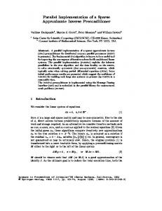
In table 1 we present the convergence results for a variety of iterative methods and decreasing values of " . The convergence results without preconditioning are listed under M = I . We denote by cgne the cg algorithm applied to the preconditioned normal equations AMM T AT y = b with x = MM T AT y. As we reduce " and kAM ? I kF , the number of iterations drops signi cantly for all iterative methods. The results in table 1 underline the robustness of the preconditioner with respect to ". In table 2 we compare dierent norms of AM ? I as a function of ". The `1 norm remains nearly constant, because as " decreases, the amount of ll-in per column in M increases. Thus, M = 0 is a better solution of the minimization problem kAM ? I k1 than the computed M for all "  0:12 . This is also true for the `2 norm as long as "  4:8 . This indicates that neither the `1 nor the `2 norm are good measures of the proximity of AM to the identity, if the Frobenius norm is being minimized. As we reduce " the singular values cluster about one, as demonstrated in theorem 3.3. This is clearly shown in table 2, since the condition number of AM is the ratio of the largest to the smallest singular value. In gure 1 we verify the improvement in the clustering of the eigenvalues predicted by theorem 3.2 as we reduce ". Next, we compare the approximate inverse M with the true inverse A?1. We computed A?1 and discarded all entries whose absolute value was less than or equal to 0.001 . Then, we computed the approximate inverse M with " = 0:36 . It is quite striking how well the sparsity patterns of both matrices agree with each other qualitatively in 13

M =I " = 0:72 " = 0:60 " = 0:48 " = 0:36 " = 0:24 " = 0:12

(M ) kAM ? I kF kAM ? I k2 kAM ? I k1 cond(AM ) nz nz(A) 6 5 5 4 1:6  10 4:6  10 5:7  10 6:3  10 | 11.4 9.58 8.02 6.80 4.75 2.52

1.02 1.07 1.04 0.97 0.93 0.74

1.56 1.56 1.56 1.56 1.70 1.28

173 168 69.0 22.7 11.0 4.15

0.57 0.79 1.11 2.10 3.89 9.69

Table 2. Oilgen3: kAM ? I k and the condition number of AM for dierent values of " .

bcg cgs bi-cgstab gmres(20) gmres(50)

oilgen1, M = I 412 229 " = 0:4 87 46 oilgen2, M = I > 1000 998 " = 0:4 70 44

378 50 > 1000 43

754 79 > 1000 83

510 77 > 1000 72

Table 3. Convergence results for oilgen1 and oilgen2: unpreconditioned (M = I ), and preconditioned (" = 0:4).

gure 2. We conclude this section with the convergence results for both oilgen1 and oilgen2. The relative ll-in nz(M )=nz(A) was 1.00 for oilgen1 and 0.94 for oilgen2.

14

0.2 0.1 0 -0.1 -0.2 0

0.2

0.4

0.6

0.8

1

1.2

0.2

0.4

0.6

0.8

1

1.2

0.2 0.1 0 -0.1 -0.2 0

Figure 1. Oilgen 3: eigenvalues of AM with " = 0:72 (top), and with " = 0:24 (bottom).

5 Numerical Examples In this section we consider a wide spectrum of problems coming from real scienti c and industrial applications. We shall demonstrate the eectiveness of the preconditioner for two standard but very dierent iterative methods: bi-cgstab and gmres with restart. We recall that the former requires two whereas the latter only one matrix-vector multiplication per iteration. In all numerical calculations the initial guess was x0 = 0, r~0 = r0 = b, and unless speci ed, the stopping criterion was as in (33). All the computations were done in Fortran and in double precision. We begin with the convergence results for the ve shermanx black oil simulators. This set consists of sherman1: a black oil simulator, shale barrier, 10  10  10 grid, 1 unknown, of size n = 1000 and with nz = 3750 nonzero elements. sherman2: a thermal simulation, steam injection, 665 grid, 5 unknowns, n = 1080 and nz = 23094. 15

0

0

200

200

400

400

600

600

800

800

0

200

400 600 nz = 19984

800

0

200

400 600 nz = 12559

800

Figure 2. Oilgen 3: sparsity pattern of entries in A?1 larger than 0.001

in absolute value (left), and sparse approximate inverse M with " = 0:36 (right).

sherman3: a black oil, impes simulation, 35  11  13 grid, 1 unknown,

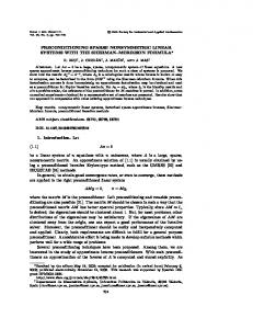
n = 5005 and nz = 20033. sherman4: a black oil, impes simulation, 16  23  3 grid, 1 unknown, n = 1104 and nz = 3786. sherman5: a fully implicit black oil simulator, 16  23  3 grid, 3 unknowns, n = 3312 and nz = 20793. Here the right-hand side was always provided. Table 4 shows that preconditioning clearly improves the convergence for all considered problems. The maximal ll-in denotes the upper limit on the number of nonzero elements per column in M . For sherman2, both bi-cgstab and gmres(20) reduced the relative residual below 10?5 after 4 and 7 steps respectively, but never reached 10?8. This may be due to the very large condition number 9:64  1011 of sherman2, and could not be improved upon in double precision. In gure 3 we have displayed both the original matrix A and the approximate inverse M for sherman2. This picture clearly shows why we cannot simply set M equal to a banded matrix like in [8]. Indeed the sparsity structures of A and M are totally dierent in this particular case, whereas the amounts of ll-in in both matrices are almost equal. 16

sh1 sh2 sh3 sh4 sh5 bi-cgstab 405 > 1000 > 1000 97 > 1000 gmres(20) > 1000 > 1000 > 1000 792 > 1000 bi-cgstab 41 4 (< 10?5 ) 72 28 41 gmres(20) 89 7 (< 10?5 ) 264 86 173 nz(M )=nz(A) 1.34 1.14 2.42 2.45 1.34 " max. ll-in 0.4 100 0.4 50 0.2 100 0.2 50 0.2 50

Table 4. Convergence results for shermanx: unpreconditioned (top), and preconditioned (bottom).

The next set of examples consists of the larger problems in the poresx and saylorx collections: pores2: a nonsymmetric matrix, n = 1224 and nz = 9613. pores3: a nonsymmetric matrix, n = 532 and nz = 3474. saylor3: a nonsymmetric problem, n = 1000 and nz = 3750. saylor4: a nonsymmetric problem, n = 3564 and nz = 22316. Here the right-hand side was chosen random. Because pores2 generated a lot of ll-in in M and never reached the relative tolerance of 10?8 , we opted for left instead of right preconditioning. Thus in the case of pores2, we considered kMA ? I kF instead of (4). Yet we still computed the exact residual of the original problem to check convergence. This approach proved to be more ecient, because the rows of A?1 could be approximated more eectively than its columns. In gure 4 we compare both pores2 and its left approximate inverse. Again the amounts of ll-in are very similar, although the sparsity patterns are quite dierent. For pores2, gmres(20) reduced the relative residual below 10?6 after 106 iterations, but did not improve any further. This may be due to the large condition number of pores2 equal to 1:1  108 . In saylor3 we discovered in columns 988, 989, 998, and 999 two independent 2  2 singular submatrices. We ignored those four columns in the computation of M , and simply replaced the two submatrices by 2  2 17

0

0

200

200

400

400

600

600

800

800

1000

1000

0

500 nz = 23094

1000

0

500 nz = 26316

1000

Figure 3. Sherman2: original matrix A (left), and sparse approximate inverse M with " = 0:4 (right).

identity matrices. To guarantee the existence of a solution, we set the righthand side to A times a random vector. The oilgenx, shermanx, poresx, and saylorx problems were all taken from the Harwell-Boeing matrix collection. A comparative study of these problems for dierent iterative methods using incomplete LU preconditioning can be found in [13]. In the nal part of this section we shall consider a selection of very large problems. The right-hand side was always provided, the initial guess x0 = 0, and the tolerance as in (33). We start with three typical problems from Centric Engineering : P1: incompressible ow in a pressure driven pipe, T = 05, n = 3242 and nz = 293409. P2: incompressible ow in a pressure driven pipe, T = 25, n = 3242 and nz = 293551. P3: landing hydrofoil airplane FSE model, n = 6316 and nz = 167178. P4: slosh tank model, n = 3402, nz = 130371. We remark that we have used the actual number of nonzero elements in the Px matrices, since about 0.3% of the entries were zero in the original data les. It is quite remarkable that although the Px matrices are rather 18

0

0

500

500

1000

1000

0

500 1000 nz = 9613

0

500 1000 nz = 10948

Figure 4. Pores2: original matrix A (left), and sparse approximate inverse M with " = 0:4 (right).

full, we obtain such a big improvement in convergence with much sparser approximate inverses. Moreover, because of the periodic pattern in gure 5, one could determine the sparsity pattern of the rst few columns of M , and then slide the pattern about the diagonal down to the lower right corner, to get the full sparsity structure. To conclude this series of numerical experiments, we consider three problems coming from an implicit 2-D Euler solver for an unstructured grid [15]. The matrices are of order n = 62424 with nz = 1717792 nonzero elements, and correspond to the initial and later stages in the ow simulation. None of the problems converged without preconditioning. The rst problem T01 was much easier, since the ow was still in its initial stage. It is also discussed in [5]. Again, we see with T01 that we obtain a considerable improvement in convergence with a very sparse approximate inverse, thanks to the automatic selection process of the SPAI algorithm. We ran T01 with " = 0:4, a max. ll-in of 50, and nz(M )=nz(A) = 0:3 . Both T25 and T50 ran with " = 0:3, a max. ll-in of 100, and nz(M )=nz(A) = 1:3.

19

pores 2 bi-cgstab > 1000 gmres(20) > 1000 bi-cgstab 78 nz(M )=nz(A) 1.14 " max. ll-in 0.4 50 bi-cgstab 27 gmres(20) 103 (< 10?6) nz(M )=nz(A) 5.16 " max. ll-in 0.2 150

pores 3 saylor 3 saylor 4 > 1000 369 > 1000 > 1000 > 1000 > 1000 118 104 285 1.17 1.29 2.02 0.4 50 0.4 50 0.3 100 118 67 67 599 69 > 1000 4.82 2.00 3.8 0.2 50 0.3 100 0.2 150

Table 5. Convergence results for poresx and saylorx: unpreconditioned

(top), and preconditioned (middle & bottom). Left preconditioner for pores2.

P1 P2 P3 P4 bi-cgstab 221 323 108 > 1000 gmres(30) > 1000 > 1000 67 > 1000 bi-cgstab 79 83 5 6 gmres(30) 866 685 10 12 nz(M )=nz(A) 0.10 0.33 0.20 0.37 " max. ll-in 0.3 50 0.25 100 0.4 100 0.4 150

Table 6. Convergence results for Px: unpreconditioned (top), and preconditioned (bottom).

20

0

0

500

500

1000

1000

1500

1500

2000

2000

2500

2500

3000

3000

0

1000 2000 nz = 293409

3000

0

1000 2000 nz = 30372

3000

Figure 5. P1: original matrix A (left), and sparse approximate inverse M with " = 0:3 (right).

6 Conclusion We have presented a new algorithm to compute a sparse approximate inverse M of a sparse, nonsymmetric matrix A. The computation of M is inherently parallel, since its columns are calculated independently of one another. The matrix M gives valuable insight into A?1, and provides a measure on the proximity of M to A?1 . Instead of imposing an a priori sparsity pattern upon M , we let the algorithm capture automatically the relevant entries in the inverse. Thus, we minimizethe amount of ll-in present in M and concentrate the computational eort where it is needed. The algorithm generates a robust and exible preconditioner for iterative solvers, as it gives full control over the ll-in and the quality of M . It is possible to minimize the total execution time for a particular problem and architecture, by choosing an optimal amount of ll-in in M . It is clear that a very sparse preconditioner is very cheap but may not lead to much improvement in convergence, and that if M becomes too dense, it becomes too expensive to compute. The optimal preconditioner lies somewhere between these two extremes, and is problem and architecture dependent. The implementation of this method on a parallel computer is straightforward, since all calculations are done independently. Yet, each processor 21

0

10

-2

10

-4

10

-6

10

-8

10

-10

10

-12

10

0

50

100

150

200

250

300

350

400

450

500

Figure 6. Convergence history of Tx with bi-cgstab: relative residual vs.

number of iterations for T01(dash-dot), T25(dotted), T50(solid).

must have access to the data required to solve its subproblem. Although the preconditioner is invariant under permutation, the ordering of the unknowns can aect the amount of inter-processor communication involved in the computation of M , and may be optimized for a particular application. This new approach will prove particularly eective when a linear system needs to be solved repeatedly, such as in implicit time-marching schemes and the solution of nonlinear equations.

7 Acknowledgements We would like to thank Horst Simon from NASA Ames for providing us with the numerical examples presented in this paper, and for his very helpful and supportive comments. 22

References [1] R. Barret et al.. Templates for the Solution of Linear Systems, SIAM, Philadelphia, 1994. [2] E. Chow, Y. Saad. Approximate Inverse Preconditioners for General Sparse Matrices, Colorado Conference on Iterative Methods, April 5-9, 1994. [3] S. Demko, W.F. Moss, and P.W. Smith. Decay Rates for Inverses of Band Matrices, Math. Comp., 43 (168), p. 491{499, 1984. [4] R.W. Freund, G.H. Golub, N.N. Nachtigal. Iterative Solution of Linear Systems, Acta Numerica p. 57-100, 1991. [5] R.W. Freund and N.N. Nachtigal. Implementation details of the coupled QMR algorithm, Numerical Linear Algebra, (L. Reichel, A. Ruttan, and R.S. Varga, W. de Gruyter, Berlin, pp. 123{140, 1993. [6] J.D.F. Cosgrove, J.C. Diaz, and A. Griewank. Approximate Inverse Preconditionings for Sparse Linear Systems, Intern. J. Computer Math. 44, p. 91{110, 1992. [7] M. Grote and H. Simon. Parallel Preconditioning and Approximate Inverses on the Connection Machine, Proceedings of the Scalable High Performance Computing Conference (SHPCC), 1992 Williamsburg, VA, IEEE Computer Science Press, p. 76{83, 1992. [8] M. Grote and H. Simon. Parallel Preconditioning and Approximate Inverses on the Connection Machine, Proceedings of Sixth SIAM Conference on Parallel Processing for Scienti c Computing II, ed. by Richard Sincovec et al., SIAM, p. 519{523, 1993. [9] L.Yu. Kolotilina and A.Yu. Yeremin. Factorized Sparse Approximate Inverse Preconditionings, SIAM J. Matrix An. Appl. 14 (1), p. 45{58, 1993. [10] L.Yu. Kolotilina, A.A. Nikishin, and A.Yu. Yeremin. Factorized Sparse Approximate Inverse (FSAI) Preconditionings for Solving 3D FE Systems on Massively Parallel Computers II, Iteritive Methods in Linear Algebra, Proc. of the IMACS International Symposium, eds. R. Beauwens and P. de Groen, Brussels, April 2-4, 1991, p. 311{312, 1992. 23

[11] Ju.B. Lifshitz, A.A. Nikishin, and A.Yu. Yeremin. Sparse Approximate Inverse Preconditionings for Solving 3D CFD Problems on Massively Parallel Computers , Iteritive Methods in Linear Algebra, Proc. of the IMACS International Symposium, eds. R. Beauwens and P. de Groen, Brussels, April 2-4, 1991, p. 83{84, 1992. [12] Y. Saad. A Flexible Inner-Outer Preconditioned gmres Algorithm, SIAM J. Sci. Stat. Comput. 14 (2), p. 461{469, 1993. [13] C.H. Tong. A Comparative Study of Preconditioned Lanczos Methods for Nonsymmetric Linear Systems, Sandia report SAND91-8240, Sandia National Laboratories, January 1992. [14] H. A. Van Der Vorst, Bi-CGSTAB: A fast and smoothly converging variant of Bi-CG for the solution of nonsymmetric linear systems, SIAM J. on Sci. and Stat. Comp., 13 (1992), no. 2, pp. 631-644. [15] V. Venkatakrishnan and T.J. Barth, Unstructured Grid Solvers on the iPSC/860, Parallel Computational Fluid Dynamics, Rutgers, New Jersey, May 1992.

24