A New Multi-Algorithm Approach to Sparse System Adaptation1 Ashrith Deshpande and Steven L. Grant2 University of Missouri-Rolla 228 EECH, 1870 Miner Circle Rolla MO 65401 email:
[email protected] ABSTRACT This paper introduces a new combination of adaptive algorithms for the identification of sparse systems. Two similar adaptive filters, proportionate normalized least mean squares (PNLMS) and exponential gradient (EG) have been shown to have initial convergence that is much faster than the classical normalized least mean squares (NLMS) when the system to be identified is sparse. Unfortunately, after the initial phase, the convergence is then actually slower than NLMS. Another algorithm developed by Gansler, Benesty, Sondhi, and Gay, which we will refer to as GBSG, operates in a manner complementary to PNLMS and EG. Its initial convergence is at about the same rate as NLMS, but gradually accelerates to a fast final convergence. By combining both algorithms, PNLMS and GBSG we obtain fast adaptation convergence rates in both initial and final phases of the process. 1. INTRODUCTION The proportionate normalized least mean squares (PNLMS) algorithm [1] is an adaptive filter whose initial convergence is much faster than the classical normalized least mean squares (NLMS) adaptive filter when the solution is sparse in non-zero terms. Developed independently, the exponentiated gradient (EG) adaptive filter [2] is very similar to PNLMS. The connection between the two algorithms was demonstrated by Benesty [3]. Unfortunately, after the initial phase, PNLMS and EG’s convergence rate becomes slower than NLMS. This problem was addressed somewhat by the introduction of PNLMS++ [4] and IPNLMS [5]. These algorithms combine PNLMS with NLMS in different ways such that
1 2
This work was funded by the Wilkens Missouri Endowment. Formerly, Steven L. Gay
Figure 1: A typical network echo canceller configuration
the initial phase convergence is like PNLMS, and the second phase convergence is like NLMS. In this paper we use yet another adaptive filter, one developed by Gansler, Benesty, Sondhi, and Gay, [6] which we will refer to as, GBSG. GBSG was mainly developed as a low complexity alternative to NLMS for use in a concentrated bank of network echo cancellers. In addition to lower complexity, GBSG has an interesting side-effect of having a faster convergence rate than NLMS, especially near convergence. Here, we are more interested in its GBSG’s convergence properties and regard it’s lower computational complexity as the sidebenefit. Since convergence behavior is complementary to PNLMS and EG, we combine the algorithms in the manner of Gay [4] to achieve fast overall convergence.
In this paper, we review PNLMS and GBSG in sections 2 and 3 respectively, discuss their combination in section 4 and give our conclusions in section 5. 2. PNLMS A typical network echo cancellation arraignment is shown in Figure 1. x ( n ) is the far-end signal which excites the echo
path
x ( n ) = ⎡⎣ x ( n ) ,
and
the
adaptive
filter.
, x ( n − L + 1)⎤⎦ is the L-length excitation T
vector. The L-length network echo path impulse response T vector, hep = [ h0 , …, hL −1 ] , is a combination of the network delays to and from the hybrid circuit, and the hybrid circuit/local loop response. Typically, the hybrid/local loop response only has about 6 ms of significant coefficients while the network delays vary over a range of 60 to 90 ms or more. This accounts for the sparse nature of the network echo cancellation problem. vn is the nearend signal, and/or near-end noise and y ( n ) = xT ( n ) hep + v ( n ) is the combination of the echo and near-end signals. h ( n ) = ⎡⎣ h0 ( n ) ,..., hL −1 ( n ) ⎤⎦ represents the T
adaptive filter coefficient vector and e ( n ) is the error or residual-echo signal. G ( n ) = diag { g 0 ( n ) , … , g L −1 ( n )} is the PNLMS diagonal individual step-size matrix, µ , is the “stepsize” parameter (chosen in the range, 0 < µ < 1 ), and δ is a small positive number known as the regularization parameter. The sample rate for all signals in this paper is 8 kHz. An NLMS adaptive filter iteration involves the following two steps: e ( n ) = y ( n ) − xT ( n ) h ( n ) , (1) the error calculation, and −1
h ( n ) = h ( n − 1) + µ x ( n ) ⎡⎣ xT ( n ) x ( n ) + δ ⎤⎦ e ( n ) ,
(2)
small that their coefficients stop adapting. This proportionate weighting can be seen as coming from a cost function that favors coefficient updates that move along a coordinate axis in the parameter space [7]. This is illustrated in Figure 2. Table 1: f ( ρ , δ p , h ( n − 1) )
Step
Calculation
a Lmax = max {δ p , h0 ( n − 1) ,…, hL −1 ( n − L + 1) } b γ i = max {ρ Lmax , hi ( n − 1) } 0 ≤ i ≤ L − 1 c
L −1
L1 = ∑ γ i i =0
d ⎡⎣G ( n ) ⎦⎤ = γ i / L1 i ,i
0 ≤ i ≤ L −1
When h ( n − 1) is sparse, it lies near a coordinate axis and the cost function makes it is cheap to move parallel to the axis and expensive to move orthogonal to it. Thus, the fast initial convergence of PNLMS occurs because of fast movements along the coordinates where h ep is large, and the slow convergence of the second phase is due to the relatively slow movements orthogonal to those large coordinate parameters. When h ep is dispersive, PNLMS has no advantage over NLMS, in fact its convergence is significantly slower. PNLMS++ [4] and IPNLMS [5] were designed to improve the convergence rate for dispersive impulse responses so that they converge at least as fast as NLMS. PNLMS++ accomplishes this by either alternating the PNLMS and NLMS updates in consecutive sample periods (PNLMS++(AU)), or by combining both types of updates in each sample period (PNLMS++(DU)).
the coefficient vector update. PNLMS is similar, except that in the coefficient vector update a diagonal matrix, G (n) , whose elements are roughly proportionate to the magnitude of the coefficient vector, h ( n − 1) , is used to window the excitation vector, x ( n ) .
The PNLMS
coefficient update is
h ( n ) = h ( n − 1) + −1
+ µ G ( n ) x ( n ) ⎡⎣ xT ( n ) G ( n ) x ( n ) + δ ⎤⎦ e ( n )
where,
G ( n ) = f ( ρ , δ p , h ( n − 1) )
(3)
(4)
and f ( ρ , δ p , h ( n − 1) ) is a nonlinear function described by the series of steps in Table 1. The parameters δ p and ρ prevent the individual step sizes from taking on values so
Figure 2: The PNLMS cost function favors movement along the coordinate axes in the parameter space
IPNLMS presents a different and more flexible way of combining the double updates of PNLMS++(DU). The coefficient error is defined as,
(
J = 20log10 h ( n ) − h ep / h ep
)
(5)
Figure 3 shows a comparison of the coefficient error convergence of PNLMS++(AU) to NLMS for the simulated network echo path whose impulse response is shown in figure 4. Here, a first order IIR filter with a pole at z=0.9 is used to simulate the hybrid/local loop response. The length of the echo path and adaptive filter is 1024 coefficients. The excitation signal, x ( n ) , is zero mean white Gaussian noise. Both NLMS and PNLMS use a stepsize of µ = 1 and a regularization parameter of δ = 1 . The near-end signal energy is set to be 40 dB below the echo signal. Here, we see the typical fast initial convergence of PNLMS++ followed by its slower second
Figure 5: Convergence of NLMS and GBSG
phase convergence. 3. GBSG
Figure 3: Convergence of NLMS and PNLMS++(AU)
GBSG [6] is a low complexity method that uses NLMS along with the idea of a set, AS of “active coefficients.” In this method, every Nth sample period a regular NLMS error calculation and coefficient update is made followed by a determination of AS . In the N-1 subsequent sample periods, NLMS is applied only to the coefficients in AS . In sparse problems the number of active coefficients, N A , is considerably smaller than L, thus reducing the computational complexity of the calculations. The set AS is determined as follows: 1.
define Ec = ∑ i = 0 hi ( n )
2.
sort the coefficients in descending order of absolute value AS is defined as the first N MAX coefficients or the first N A coefficients in the list whose cumulative sum just exceeds T • Ec , which ever is smaller
3.
L −1
Typically, 0.9 ≤ T < 1 and for L=1000, N MAX ≈ 100 . The error calculation and coefficient update of the active coefficients is, e ( n ) = y ( n ) − xT ( n ) WA ( n ) h ( n )
and
(6)
h ( n ) = h ( n − 1) + −1
+ µ WA ( n ) x ( n ) ⎡⎣ xT ( n ) WA ( n ) x ( n ) + δ ⎤⎦ e ( n )
Figure 4: Impulse response of the simulated network echo path
(7)
where
{W ( n )} A
ii
⎧1 i ∈ AS =⎨ ⎩0 i ∉ AS
(8)
Figure 5 shows a comparison of convergence curves for NLMS and GBSB for N=10 and T=0.98 where the salient parameters are the same as those used in the previous simulation description. As advertised, GBSG initially converges at about the same rate as NLMS, but gradually accelerates toward final convergence. 4. PNLMS Combined with GBSG We combine PNLMS and GBSG in the same manner that PNLMS and NLMS are combined in PNLMS++(AU), that is alternating the two forms of updates in subsequent sample periods. Another way of describing the combination is that we replace the full NLMS updates in GBSG with PNLMS updates and then set N=2. With this combination, the initial fast convergence of PNLMS is preserved since the updates move quickly parallel to the coordinate axes in the parameter space where the h ep coefficients are large. Then, when normally, the small, but still not insignificant coefficients of h ( n ) begin to converge, their convergence is mainly determined not by an L-length NLMS update as in PNLMS++(AU), but by the shorter (and hence faster) N MAX (or shorter)-length update of Eq. (7). The convergence behavior of the resulting algorithm is shown in figure 6. Its convergence exceeds both NLMS and PNLMS++. 5. Conclusions
REFERENCES [1] D. L. Duttweiler, “Proportionate normalized leastmean-squares adaptation in echo cancellers,” IEEE Trans. Speech Audio Processing, vol. 8, pp. 508-518, Sept. 2000 [2] J. Kivinen and M. Warmuth, “Exponentiated gradient versus gradient descent for linear predictors,” Inform. Comput., Vol. 132, pp. 1-64, Jan. 1997 [3] J. Benesty and Y. Huang, “The LMS, PNLMS, and exponentiated gradient algorithms,” Proc. EUSIPCO, 2004 [4] S. L. Gay, “An efficient, fast converging adaptive filter for network echo cancellation,” Proc. of Asilomar Conf. on Signals, Systems and Comp., Nov. 1998. [5] J. Benesty and S. L. Gay, "An improved PNLMS algorithm," IEEE Int. Conf. on Acoustics, Speech and Signal Processing, May, 2002 [6] T. Gaensler, J. Benesty, M. M. Sondhi, and S. L. Gay, “Dynamic resource allocation for network echo cancellation,” in IEEE Int. Conf. on Acoustics, Speech and Signal Processing, May, 2001 [7] S. L. Gay, S. C. Douglas, “Normalized natural gradient adaptive filtering for sparse and non-sparse systems,” Proc. IEEE Int. Conf. on Acoustics, Speech and Signal Processing, May 2002
In this paper we have presented a new adaptive filtering algorithm for sparse systems that combines two coefficient updates that have complementary properties: PNLMS, which has fast initial convergence and slow final convergence, with GBSG, which has relatively slow initial convergence and fast final convergence. Together, they yield an adaptive filter that, to our knowledge, has the fastest convergence to date for sparse systems.
Figure 6: Convergence behavior of NLMS, PNLMS++(AU), and GBSG+PNLMS