merged operation in which multiple data outputs from per- vious operations ... Most coarse-grained reconfigurable arrays arrange their .... reconfigurable unit composed of an ALU, an array multip- lier, etc. .... In the first case ..... Equivalent. Area.
11th EUROMICRO CONFERENCE on DIGITAL SYSTEM DESIGN Architectures, Methods and Tools
A New Array Fabric for Coarse-Grained Reconfigurable Architecture Yoonjin Kim and Rabi N. Mahapatra Embedded Systems & Co-Design Group, Dept. of Computer Science Texas A&M University, College Station, TX 77843 {ykim, rabi}@cs.tamu.edu new reconfigurable array fabric and its hardware implementation.
Abstract Coarse-grained reconfigurable architectures (CGRA) employ square or rectangular arrays composed of many computational resources for high performance. Though these array fabrics are mostly suitable for embedded systems including multimedia applications, they occupy large area and consume much power. Therefore, reducing area and power of CGRA is necessary for the reconfigurable architectures to be used as a competitive IP core in embedded systems. In this paper, we propose a new array fabric for designing CGRA to reduce area and power consumption without any performance degradation. This costeffective approach is able to reduce the array size through efficient arrangement of array components and their interconnections. Experimental results show that for multimedia applications, the proposed array fabric reduces area up to 40.32% and saves power by up to 28.35 % when compared with the existing CGRA architecture.
The paper has following contributions: A new array fabric design exploration method has been proposed to generate cost-effective reconfigurable array structure.
•
Novel rearrangement of processing elements and their interconnection designs are introduced for CGRA to reduce area and power consumption without any performance degradation.
•
Gate level design and simulation were carries out with real application benchmarks that demonstrate the cost-effectiveness of new array fabric to reduce both the area and power consumptions.
This paper is organized as follows. After the related work in Section 2, we present the motivation of our approach in Section 3. In Section 4, we describe the new array fabric exploration flow to generate cost-effective array fabric with suitable illustrations. Then application-mapping example is shown in Section 5 and the experimental results are given in Section 6. Finally we conclude the paper in the Section 7.
1. Introduction Application-specific optimization of embedded system becomes inevitable to satisfy the market demand for designers to meet tighter constraints on cost, performance and power. On the other hand, the flexibility of a system is also important to accommodate the short time-to-market requirements for embedded systems. To compromise these incompatible demands, coarse-grained reconfigurable architecture (CGRA) has emerged as a suitable solution for embedded systems [1]. CGRA not only boosts the performance by adopting specific hardware engines but it can also be reconfigured to adapt different characteristics of class of applications. Therefore, CGRA has higher performance level than general purpose processor and wider applicability than ASIC.
2. Related works Many CGRA based systems have been proposed with increasing interests in reconfigurable computing recently [1]. Among those, the square/rectangular mesh architectures have the advantage of rich communication resources for parallelism. Morphosys [2] consists of 8x8 array of Reconfigurable Cell coupled with Tiny_RISC processor. The array performs 16-bits operations including multiplication in SIMD style. It shows good performance for regular code segments in computation intensive domains but requires large amount of area for its implementation. XPP configurable system-on-chip architecture [3] is another example. XPP has 4 x 4 or 8 x 8 reconfigurable array and LEON processor with AMBA bus architecture. A processing element of XPP is composed of an ALU and some registers. Since the processing elements do not include heavy resources, the total area cost is not high but the range of applicable domains is restricted.
In spite of the above advantages, the deployment of CGRA is prohibitive due to its significant area and power consumption. This is due to the fact that CGRA is composed of several memory components and the array of many processing elements including ALU, multiplier and divider, etc. Specially, processing element (PE) array occupies most of the area and consumes most of the powers in the system to support flexibility and high-performance. Therefore, reducing area and power consumption in the PE array has been a serious concern for their cost and reliability. For cost-effective CGRA design, this paper provides a
978-0-7695-3277-6/08 $25.00 © 2008 IEEE DOI 10.1109/DSD.2008.67
•
Most design space exploration techniques previously suggested are limited to the configuration of the internal structure of a PE and the interconnection scheme. Such configu584
Authorized licensed use limited to: IEEE Xplore. Downloaded on April 29, 2009 at 17:41 from IEEE Xplore. Restrictions apply.
ration techniques are in general good at obtaining high performance but require high area cost. To alleviate this problem, some templates permit heterogeneous PEs [4][5]. However, such heterogeneity bears strict constraints on mapping of applications to PEs, resulting in diminished performance. In addition, [4] and [5] do not change the array fabric itself by the root - architecture template is configured but keeps square/rectangular array fabric. In [6] the authors have proposed energy-aware interconnection exploration to minimize energy by changing the topology between global register file and function units. However, this exploration only provides the trade-off between performance and energy while keeping fundamental square/rectangular array fabric intact. In [7][8], authors have emphasized that the implemented architectures are power-efficient compared with fine-grained architecture such as FPGA in specific applications but the architectures only support limited some applications with low power.
3.2 Redundancy in conventional CGRA Most coarse-grained reconfigurable arrays arrange their processing elements (PEs) as a square or rectangular 2-D array with horizontal and vertical connections, which support rich communication resources for efficient parallelism. However, square/rectangular array structures have many redundant or unutilized PEs during the executions of applications onto the array. Figure 2 shows an example of three types of data flow (Figure 1) mapped onto 8x8 square reconfigurable arrays. All the three types of implementations show lots of redundant PEs that are not used. It shows the existing square/rectangular array fabric cannot efficiently utilize all of PEs on the array and therefore will waste large area and power. In order to overcome such wastages in square/rectangular array fabric, we propose a new cost effective array fabric in this paper.
3. Motivation 3.1 Characteristics of computation-intensive and data-parallel applications. Most of the CGRAs have been designed to satisfy the performance of a range of applications in particular domain. Specially, it is most applicable for applications that exhibit the computation-intensive and data-parallel characteristics. Common examples for such applications are digital signal processing (DSP) applications like audio signal processing, audio compression, digital image processing, video compression, speech processing, speech recognition, and digital communications. Such applications have many subtasks such as trigonometric functions, filters and matrix/vector operations and they are run onto coarse-grained reconfigurable array. OP1 OP2
OP4
OP4
OP1
OP2
OP5
OP2
OP3
OP6
OP3
(a) Merged
PE
PE
PE
PE
PE
PE
PE
In[0]
PE
PE
PE
PE
PE
PE
PE
PE
Out[0]
PE
PE
PE
PE
PE
PE
PE
PE
In[1]
PE
PE
PE
PE
PE
PE
PE
PE
Out[1]
In[2]
PE
PE
PE
PE
PE
PE
PE
PE
In[2]
PE
PE
PE
PE
PE
PE
PE
PE
Out[2]
In[3]
PE
PE
PE
PE
PE
PE
PE
PE
In[3]
PE
PE
PE
PE
PE
PE
PE
PE
Out[3]
In[4]
PE
PE
PE
PE
PE
PE
PE
PE
In[4]
PE
PE
PE
PE
PE
PE
PE
PE
Out[4]
In[5]
PE
PE
PE
PE
PE
PE
PE
PE
Out[5]
In[6]
PE
PE
PE
PE
PE
PE
PE
PE
In[7]
PE
PE
PE
PE
PE
PE
PE
PE
Out
In[0]
PE
PE
PE
PE
PE
PE
PE
PE
Out[0]
In[1]
PE
PE
PE
PE
PE
PE
PE
PE
Out[1]
In[2]
PE
PE
PE
PE
PE
PE
PE
PE
Out[2]
In[3]
PE
PE
PE
PE
PE
PE
PE
PE
Out[3]
In[4]
PE
PE
PE
PE
PE
PE
PE
PE
Out[4]
In[5]
PE
PE
PE
PE
PE
PE
PE
PE
Out[5]
In[6]
PE
PE
PE
PE
PE
PE
PE
PE
Out[6]
In[7]
PE
PE
PE
PE
PE
PE
PE
PE
Out[7]
In[5]
PE
PE
PE
PE
PE
PE
PE
PE
In[6]
PE
PE
PE
PE
PE
PE
PE
PE
Out[6]
In[7]
PE
PE
PE
PE
PE
PE
PE
PE
Out[7]
(b) Butterfly operation
PE : used processing element PE : not used processing element
(c) Merged butterfly operation
OP6
Figure 2. Data flow on 8x8 reconfigurable array.
OP4
(b) Butterfly
PE
(a) Merged operations
OP6 OP5
OP3
OPi
OP1
In[0] In[1]
4. New cost-effective CGRA
OP7
(c) Merged butterfly
In order to devise cost-effective coarse-grained reconfigurable array, we propose a new array fabric exploration flow as shown in Figure 3. This exploration starts from analysis of general square array fabric. New array fabric is partially derived by analyzing intra-half column connectivity of square fabric in Phase I. Then Phase II elaborates new array fabric by analyzing inter-half column connectivity of square fabric. Finally, the connectivity of new array fabric is enhanced by adding vertical and horizontal global bus. In subsection 4.1 through subsection 4.4, we describe more detailed process for each stage in entire exploration flow.
: operation
Figure 1. Subtask classification. We have classified such subtasks into three types of data flow graphs as in Figure 1. The type (a) in Figure 1 shows merged operation in which multiple data outputs from pervious operations are used as input data for next set of operations. Type (b) shows butterfly operation where multiple output data from previous operations are fed as input data to the same number of next stage operations. Finally, type (c) shows combination of (a) and (b) where an intermediate stage of operations exists for merging and de-merging operations. 585
Authorized licensed use limited to: IEEE Xplore. Downloaded on April 29, 2009 at 17:41 from IEEE Xplore. Restrictions apply.
General Square Reconfigurable Array Fabric
Global connectivity Interconnection structure in column direction
Analysis of Intra-Half Column Connectivity New Array Fabric Derivation – Phase I Analysis of Inter-Half Column Connectivity
PE
PE
PE
PE
PE
PE
PE
PE
PE
PE
Interconnection structure in row direction Frame Buffer
PE
PE
PE
PE
PE
PE
PE
PE
PE
PE
PE
PE
PE
PE
PE
PE
New Array Fabric Derivation – phase II CE
CE
Connectivity Enhancement
PE PE
PE
Cost-Effective Reconfigurable Array Fabric
PE CE
CE
PE CE
CE
PE
PE
PE CE
CE
PE
PE
PE
PE CE
CE
PE
PE CE
CE
Figure 3. Overall exploration flow.
PE
PE
PE
PE CE
CE
PE
PE CE
CE
PE
4.1 Input reconfigurable array fabric
PE
CE
PE CE
PE CE
PE CE
PE CE
PE CE
PE CE
PE CE
PE
CE
PE CE
PE CE
PE CE
PE CE
PE CE
PE CE
PE CE
PE
CE
PE CE
PE CE
PE CE
PE CE
PE CE
PE CE
PE CE
PE
CE
PE CE
PE CE
PE CE
PE CE
PE CE
PE CE
PE CE
PE
CE
PE CE
PE CE
PE CE
PE CE
PE CE
PE CE
PE CE
PE
CE
PE CE
PE CE
PE CE
PE CE
PE CE
PE CE
PE CE
PE
Pairwise connectivity
Square reconfigurable array fabric is used for input of the proposed exploration flow. A general mesh-based 8x8 reconfigurable array given in Figure 4 is used here to illustrate the proposed exploration flow. Each PE is a basic reconfigurable unit composed of an ALU, an array multiplier, etc. and the configuration of each PE is controlled by a CE (cache element). In addition, we assume that computation model of the 8x8 array is SIMD in row direction [2] or loop pipelining based on temporal mapping [9] for high performance - each iteration of application kernel (critical loop) is mapped onto each column of square array. Therefore, in this example array, columns have more interconnection than rows. The interconnection in rows is only used for the operations from inter-loop iteration. In the case of pair-wise interconnection, column and row have nearestneighbor and hopping interconnections like Figure 4. In addition, each column has 2 global buses and each row shares two read-buses and one write-bus.
Figure 4. Example of square reconfigurable array. In Phase I, new array fabric is initially constructed by analyzing intra-half column connectivity of the input square array. Algorithm 1 shows this procedure. Algorithm 1 New Array Fabric Derivation – Phase I L1 L2
base ← a half column of n x n reconfigurable array m ← number of memory-read buses of n x n reconfigurable array
L3
new_array_space ← Ø
L4
begin
L5 L6
source_column_group ← Add a column composed of n/2 PEs in new_array_space while CHECK_PAIR-WISE(source_column_group, base) do
L7
Add two PEs in new array_space
L8
LOC_RHT-TRI(added PEs, source_column_group)
L9
end do
L10
source _column_group ← Ø
L11
source _column_group ← next two columns on the both sides
L12
if |source-column_group| > 2 then
4.2 New array fabric derivation – Phase I
in new_array_space
1
Interconnection fabric among PEs in the same column can be classified into intra-half and inter-half column connectivity. Intra-half column connectivity means pair-wise interconnection between PEs in a half column and Interhalf column connectivity means pair-wise interconnection or global bus between PEs – one PE is included in a half column and another PE is included in other half column.
L13
goto L6
L14
end if
L15
Add nearest-neighbor interconnections
L16
Add m memory-read buses
L17
Connect the read buses with the added PEs in the same row
L18 L19
Copy the constructed fabric on vertically symmetric position end
Before we explain the procedure in detail, we introduce notations we use in the explanation.
1
y (L1) base denotes base column that is a half column of n x n reconfigurable array. y (L3) new_array_space denotes 2-dimentional space for cost-effective reconfigurable array. y (L5) source_column_group denotes column group composed of one or two source columns in new_array_space. It is used as source for derive new array fabric.
We do not consider interconnection in rows of square array for generating new array fabric. This is because application kernels are spatially mapped onto new array fabric. It means that result data from each loop iteration converges into a PE.
586
Authorized licensed use limited to: IEEE Xplore. Downloaded on April 29, 2009 at 17:41 from IEEE Xplore. Restrictions apply.
y (L12) |source_column_group| denotes the number of PEs in source_column_group. y (L6) CHECK_PAIR_WISE is a function to identify pairwise interconnections of PEs in source_column_group by analyzing base column. y (L8) LOC_RHT_TRI means local-right triangular method that is a function to assign added PEs new positions in new_array_space and connect them with the PEs in source column.
back to the central column that is directly added from the base column. Figure 6 shows two examples on how to find pair-wise connectivity on source columns. In the case of (a) of Figure 6, no interconnection between ‘PE4’ and ‘PE6’ (or ‘PE7’ and ‘PE9’) is added because there is no hopping connectivity between ‘PE0’ and ‘PE2’ (or ‘PE0 (or 1)’ and ‘PE3’). However, in the case (b), Figure 6 the base column has interconnection between ‘PE0’ and ‘PE2’. Therefore interconnections between ‘PE4’ and ‘PE6’ (or ‘PE7’ and ‘PE9’) are added by local right-triangular method.
The algorithm starts with initialization step (L1~L3). Then a half column is added in new array space and it is initial source_column_group (L5). Next process is to check the pair-wise connectivity between two PEs (L6) – two PEs in the same column included in source_column_group. This checking process (L6) continues until no more pair-wise interconnection is found. PE PE
PE0 PE1
PE PE
PE
PE
PE4
PE8
PE2
PE5
PE
PE3
PE
PE9
PE3
PE6
PE
(a) Nearest-neighbor PE0
PE
PE
PE1
PE
PE0
PE1 PE2
PE
PE7
PE2
PE
(a) Nearest-neighbor PE
PE0
PE7
PE1
PE4
PE
PE8
PE2
PE5
PE
PE
PE9
PE3
PE6
PE
PE PE
PE3
PE
(b) Hopping PE : PE in base column
PE : PE in source_column_group
(b) Hopping
PE : Added PE
Figure 5. Local right-triangular method. The first checking process is performed by simply identifying pair-wise interconnections of base. If a pair-wise interconnection is found, two PEs are added in new_array_space and their interconnections and positions are assigned by local right-triangular method (L8) to guarantee butterfly operation on new reconfigurable fabric. Figure 5 shows two cases of the method. In the first case (a), two PEs in base column have nearest-neighbor interconnection, which means maximum two PEs can be used for butterfly operation. Therefore, local right-triangular method assigns each PE the nearest-neighbor position on each side of the source column and the positions are vertices of right-triangular. Then the method assigns nearestneighbor interconnection between added PEs and the PEs in the source_column_group. The second case (b) shows that two PEs in base column have hopping interconnection. Local right-triangular method is also applied to this case with hopping interconnections instead of the nearest neighbor interconnections for the first case.
PE : PE in base column
PE : PE in source_column_group
: already connected
PE : Added PE
PE : preoccupied PE in new array space
: Added interconnection
Figure 6. Interconnection derivation. After the iteration of adding PEs and interconnections (L5~L14) is finished, nearest-neighbor interconnections are added between two nearest-neighbor PEs that are not connected with each other. It is to guarantee the minimum data-mobility for data rearrangement (L15). Finally, 2memory-read buses are added (L16, L17) and the derived array is copied to the vertically symmetric position (L18). Example: Figure 7 shows the result of the phase I procedure for an example of 8x8 reconfigurable array considered in section 4.1.
4.3 New array fabric derivation – Phase II In Phase II, new PEs and interconnections are added for reflecting intra-half column connectivity of the input square
From second checking process, preoccupied columns are included in source_column_group. Therefore it is necessary to find pair-wise connectivity on source column by tracing
2
Memory write-buses are added in the step of connectivity enhancement (section 4.4.) This is because some PEs can be added in phase II and they should be connected to memory-write buses.
587
Authorized licensed use limited to: IEEE Xplore. Downloaded on April 29, 2009 at 17:41 from IEEE Xplore. Restrictions apply.
In the case of pair-wise interconnection, Algorithm 1 in section 4.2 is used with slight modifications. The modifications are as follows.
fabric. Phase II analyzes two kinds of interconnections – pair-wise and global bus. PE
y (L1) base ← an entire column of n x n reconfigurable array y (L5) source_column_group ← central column in Phase I
PE
PE
PE
PE
PE
PE
PE
PE
PE
PE
PE
PE
PE
PE
PE
PE
PE
PE
PE
PE
PE
PE
PE
PE
PE
PE
PE
PE
PE
PE
PE
PE
PE PE PE PE PE PE
y L2, L3, L15, L16, L17, L18 are skipped. In the case of global bus, we propose another procedure as Algorithm 2. Before we explain the procedure in detail, we introduce notations we use in the explanation. y (L5) CHECK_GLOBAL_BUS is a function to identify bus-connectivity between two PEs in the source column. y (L6) GB_RHT_TRI means global-right triangular method that is a function used to add global buses and global PEs.
PE
(a) Two base columns (b) Nearest-neighbor interconnection
Algorithm 2 New Array Fabric Derivation - Phase II : Global Bus
PE PE
PE
PE
L1 L2
base ← a column of n x n reconfigurable array n ← number of global buses
L3
begin
L4
source_column_group ← central column in new_array_space
L5
while CHECK_GLOBAL_BUS(source_column_group, base) do
L6
PE
PE
PE
PE
PE
PE
PE
PE
PE
PE
PE
PE
GB_RHT_TRI (source_column)
L7
end do
L8
source _column_group ← Ø
L9
source _column_group ← next two columns on the both sides
L10
if |source-column_group| > 2 then
in new_array_space
PE
PE
PE
PE
PE
PE
PE
PE
PE
PE
PE
PE
PE
PE
L11
PE
L12 L13
(c) Hopping interconnection
PE
Frame Buffer
PE
PE
PE
PE
PE
PE
PE
PE
PE
PE
PE
PE
PE
PE
PE
PE
PE
PE
PE
PE
PE
PE
PE
PE
PE
PE
PE
PE
PE
end
The algorithm starts with initialization step (L1, L2). Then central column in new_array_space is initial source_column_group. Next process is to check the global bus-connectivity between two PEs (L5) - two PEs in the same column included in source column group. If two PEs have already pair-wise interconnection, global bus is not used for the PEs. Otherwise, global buses are added by global-right triangular method. This checking process (L5) continues until no more global bus-connectivity is found. Figure 8 shows two cases of global-right triangular method when base column has two global buses supporting butterfly operation. In the case of (a), two diagonal lines from two PEs in source column intersect on already existing PE called ‘destination PE’. Therefore, three global buses are added and they connect destination PEs with PEs in source column. However, in the case of (b), no destination PE exists on intersection point of two diagonal lines. Therefore, new PEs called global PE (GPE) as well as global buses are added on new_array_space.
PE
PE
goto L5 end if
PE
(d) Memory read-buses Figure 7. New array fabric example by Phase I.
588
Authorized licensed use limited to: IEEE Xplore. Downloaded on April 29, 2009 at 17:41 from IEEE Xplore. Restrictions apply.
PE PE
PE
PE
PE
PE
PE
PE
PE
PE
PE
PE
PE
PE
PE
PE
PE
PE
PE
PE
PE
PE
PE
PE
PE
PE
PE
PE
PE
PE
PE
PE
PE
PE
PE
PE
PE
PE
PE
PE
PE PE PE
PE
PE
PE
PE
PE
PE
PE
PE
PE
PE PE
PE
PE
(a) When destination PE exists
(a) Pair-wise interconnection PE
PE GPE
GPE
PE
PE
PE
PE
PE
PE
PE
PE
PE
PE
PE
PE
PE
PE
PE
PE
PE
PE
PE
PE
PE
PE
PE
PE
PE
PE
PE
PE
PE
PE
PE
PE
PE
PE
PE
PE
?
?
PE
GPE
PE
PE
PE
PE
PE
PE
PE
PE
PE
PE
PE
PE
PE
PE
PE
PE
PE
PE
PE
PE
PE
PE
PE
PE
PE
PE
PE
PE
PE
PE
PE
PE
PE
PE
PE
PE
GPE
PE
PE
GPE
PE
GPE
PE
PE
(b) Global bus interconnection
(b) When GPE is added Figure 9. New array fabric example by phase II. PE : PE in source_column_group
PE : destination PE
? : destination PE does not exists GPE : added Global PE
: added grobal bus : connection between PE and bus
Figure 8. Global right-triangular method when n = 2 (L2).
PE
PE
PE
PE
PE
PE
PE
PE
PE
PE
PE
PE
PE
PE
PE
PE
PE
PE
PE
PE
PE
PE
PE
PE
PE
PE
PE
PE
PE
PE
PE
PE
PE
PE
PE
PE
PE
GPE
Example: Figure 9 shows the result of the phase II procedure for an example of 8x8 reconfigurable arrays.
4.4 Connectivity enhancement Finally, vertical and horizontal bus can be added to enhance connectivity of new reconfigurable array. This is because new array fabric from phase I and II only has pair-wise interconnection in vertical and horizontal direction whereas it supports sufficient diagonal connectivity. Added horizontal bus is used as memory-write bus connected with frame buffer as well as used for data-transfer between PEs.
Frame Buffer
PE
GPE
Example: Figure 10 shows the result of the connectivity enhancement for an example of 8x8 reconfigurable array. Each bus is shared by two PEs in both the sides.
.
GPE
PE
GPE
PE
Figure 10. New array fabric example by connectivity enhancement.
589
Authorized licensed use limited to: IEEE Xplore. Downloaded on April 29, 2009 at 17:41 from IEEE Xplore. Restrictions apply.
for gate-level simulation and power estimation. To obtain the power consumption data, we have used the kernels in Table 2 for simulation with operation frequency of 70MHz and typical case of 1.8V Vdd and 27℃.
5. Application mapping: Example Figure 11 shows an application mapping on new array fabric example generated from the exploration flow proposed in Section 4. The application considered here is the sum of absolute differences (SAD) function. Loop iteration for SAD is given in Eqn. 1. SAD
=
8
∑
a [i] − b[i]
i=1
6.2 Results 6.2.1 Area cost evaluation
(1)
Table I shows area cost evaluation for the two cases. In the Case#1, the area cost of new array is reduced by 29.31% because it has less PEs than 8x8 square array. In the case of 16x16 square array (case#2), the area reduction ratio has increased compared to the Case#1. This is because the number of PEs is also relatively more reduced than the Case#1. Therefore, the proposed approach can reduce much area cost when array size increases.
First, the operand data (a[i], b[i]) are loaded onto 8 PEs in the central column and then the left part of new reconfigurable array is used for equation 1. Each PE executes a fixed operation with static configuration. This requires the loop body to be spatially mapped onto the reconfigurable array whereas each PE executes multiple operations by changing the configuration dynamically within a loop on the square array supporting SIMD [2] or temporal loop pipelining [9]. Even though such a mapping on new reconfigurable array may have spatial limitation, rich communication resources specified by the proposed exploration flow overcome limited spatiality. In this example, nearest-neighbor interconnections and global buses are efficiently used for datatransfer and the new array has the same performance (number of execution cycles) compared with the square array.
Table 1. Area cost comparison Number of PEs base_8 x 8 64 Case#1 proposed_1 44 base_16x16 256 Case#2 proposed_2 148 Array
Gate Equivalent 630143 445448 2520432 1504194
Area Reduced(%) 29.31 40. 32
1
sub 2
2
abs
abs 3
add 5
add 4
add
3
add
4
add 3
add
2
abs 2
abs
Table 2. Power comparison.
1
sub 1
sub 1
sub
Power (mW) Reduced (%) base_8x8 proposed * First_Diff 201.07 149.90 25.45 * Tri- Diagonal 190.75 140.43 26.38 * State 198.37 148.54 25.12 * Hydro 190.86 138.89 27.23 * ICCG 164.42 121.14 26.32 ** Inner Product 200.09 149.31 25.38 ** 24-Taps FIR 174.38 125.12 28.25 Matrix-vector multiplication 163.25 121.64 25.49 Mult in FFT 187.68 134.68 28.24 Comlex Mult in AAC decoder 222.14 159.65 28.13 ITRANS in H.264 decoder 198.32 147.81 25.47 DCT in H.263 encoder 212.25 158.51 25.32 IDCT in H.263 encoder 208.99 154.02 26.30 SAD in H.263 encoder 181.22 132.29 27.00 Quant in H.263 encoder 199.38 147.30 26.12 Dequant in H.263 encoder 196.97 141.13 28.35 *Livermore loops benchmark [13], **DSPstone [14]
sub : substract-operation
Kernels
abs : absolute-operation add : add-operation op : final result
PE
i
PE
PE
2
abs
1
op : operation executed at ith cycle
sub PE : unused PE
3
add 2
abs
2
abs 2
abs
1
sub 1
: data transfer using global bus : data transfer using pair-wise interconnection
sub 1
sub
Figure 11. SAD-mapping example on new array fabric.
6. Experiments and results 6.1 Experimental setup We have implemented entire exploration flow in Figure 3 with C++. The implemented exploration flow generated the specification of new reconfigurable array fabric. For quantitative evaluation, we have designed two base arrays and two proposed arrays at RT-level using VHDL – conventional 8x8 square array like Figure 4, extended 16x16 square array and two new arrays derived from 8x8/16x16 array fabric. The architectures have been synthesized using Design Compiler [10] with TSMC 0.18 ㎛ technology [11]. ModelSim [12] and PrimePower [10] tools have been used
6.2.2 Power evaluation Table 2 shows the comparison of power consumptions between the two reconfigurable arrays: the base 8x8 square array and the proposed new array. The two arrays have been implemented without any low power technique to evaluate their power savings. Sixteen different kernels from several application domains were considered to estimate the power consumptions. It is shown that compared to the square array, the proposed array structure derived here could save up to 28.35% of the power. It has been possible
590
Authorized licensed use limited to: IEEE Xplore. Downloaded on April 29, 2009 at 17:41 from IEEE Xplore. Restrictions apply.
to reduce power consumption in the proposed array fabric by using less number of PEs to do the same job compared to the base reconfigurable array. For larger array sizes, the power saving will further increase due to significant reduction in unutilized PEs.
[2] Hartej Singh, Ming-Hau Lee, Guangming Lu, Fadi J. Kurdahi, Nader Bagherzadeh, and Eliseu M. Chaves Filho, “MorphoSys: an integrated reconfigurable system for data-parallel and computation-intensive applications,” IEEE Trans. on Computers, vol. 49, no. 5, pp. 465-481, May 2000. [3] Jurgen Becker and Martin Vorbach, “Architecture, memory and interface technology integration of an indutrial/academic configurable sys-tem-on-chip (CSoC),” in Proc. of IEEE Computer Society Annual Symp. on VLSI, 2003. [4] Nikhil Bansal, Sumit Gupta, Nikil D. Dutt, and Alex Nicolau, “Analysis of the performance of coarse-grain reconfigurable architectures with different processing element configurations,” in Proc. of Workshop on Application Specific Processors, Dec. 2003. [5] Reiner Hartenstein, M. Herz, T. Hoffmann, and U. Nageldinger, “KressArray Xplorer: a new CAD environment to optimize reconfigurable datapath array architectures,” in Proc. of ASP-DAC, 2000 [6] Andy Lambrechts, Praveen Raghavan, Murali Jayapala, “Energy-Aware Interconnect-Exploration of coarse-grained reconfigurable processors,” in Proc. of Workshop on Application Specific Processors, Sept. 2005. [7] Sami Khawam, Tughrul Arslan, and Fred Westall, “Synthesizable reconfigurable array targeting distributed arithmetic for system-on-chip applications,” in Proc. of IEEE Int. Parallel & Distributed Processing Symp., p. 150, April 2004. [8] Francisco Barat, Murali Jayapala, Tom Vander Aa Henk Corporaal, Geert Deconinck, and Rudy Lauwereins, “Low power coarse-grained reconfigurable instruction set processor,” in Proc. of Int. Conf. on Field Programmable Logic and Applications, pp. 230-239, Sept. 2003. [9] Jong-eun Lee, Kiyoung Choi, and Nikil D. Dutt, "Mapping loops on coarse-grained reconfigurable architectures using memory operation sharing," in Technical Report 02-34, Center for Embedded Computer Systems(CECS), Univ. of California Irvine, Calif., 2002. [10] Synopsys Corp. : http://www.synopsys.com [11] Taiwan Semiconductor MC’.: http://www.tsmc.com [12] Model Technology Corp. : http://www.model.com [13] http://www.netlib.org/benchmark/livermorec [14] http://www.ert.rwth-achen.de/Projekte/Tools/DSPSTONE
6.2.3 Performance evaluation The synthesis results show that the four reconfigurable arrays above have same critical path delay - 12.87 ns. It indicates the proposed approach does not cause performance degradation in terms of the critical path delay. In addition, the execution cycle count of each kernel on new array does not vary from the base square array because the functionality of the proposed architecture is same as the base model. It also indicates the cost-effectiveness of the array fabric does not come by performance degradation in terms of the execution cycle count.
7. Conclusion Coarse-grained reconfigurable architectures are considered to be appropriate for embedded systems because it can satisfy both flexibility and high performance as needed. Most reconfigurable architectures have square/rectangular array fabric composed of computational processing elements for parallel execution of multiple operations but such designs occupy huge area and consume much power. To overcome the limitations, we suggest a novel reconfigurable array fabric optimized for computation-intensive and data-parallel applications. It has been shown the new array fabric is derived from a standard square-array using the exploration flow technique proposed in this paper. The exploration flow efficiently rearranges PEs with reducing array size and change interconnection scheme to save area and power. Experimental results show that the proposed approach saves significant area and power compared to conventional base model without performance degradation. Implementation of sixteen kernels from several application domains on the new array fabric demonstrates consistent results. The area reduction up to 40% and the power savings up to 28% are evident when compared with the conventional array architecture.
References [1] Reiner Hartenstein, “A decade of reconfigurable computing: a visionary retrospective,” in Proc. of Design Automation and Test in Europe Conf., pp. 642-649, Mar. 2001.
591
Authorized licensed use limited to: IEEE Xplore. Downloaded on April 29, 2009 at 17:41 from IEEE Xplore. Restrictions apply.