The fast beamformer real-time processing engine consumes less than 2% ... A new definition of the constrained optimization criteria for achieving ... one-dimensional search. Once the ..... ments, New York: American Institute of Physics, 1995.
A NEW BEAMFORMER DESIGN ALGORITHM FOR MICROPHONE ARRAYS Ivan Tashev and Henrique S. Malvar Microsoft Research One Microsoft Way, Redmond, WA 98052, USA
ABSTRACT This paper presents a generic beamformer design algorithm for arbitrary microphone array geometry. It makes efficient use of noise models for ambient and instrumental and microphone directivity patterns. By using a new definition of the target criterion and replacing a multi-dimensional optimization with a much simpler one-dimensional search, we can compute near-optimal solutions in reasonable time. The designed beams achieve noise suppression levels between 10 and 15 dB, for microphone arrays with four to eight elements, and linear and circular geometries. The fast beamformer real-time processing engine consumes less than 2% of the CPU power of a modern personal computer, for a four-microphone array.
1. INTRODUCTION Algorithms for beamformer design with optimal noise suppression initially were based on finding of parametric solutions, given the microphone array geometry. To reduce complexity, later designs are based on finding near-optimal solutions for different target criteria; well-known algorithms include constant directivity beamformer, minimum-variance distortionless response (MVDR), linearly-constrained minimum variance (LCMV), general side lobe cancellers, and others [1], [2]. In practice, measured parameters of microphone arrays [3] differ from theoretical estimations, leading to a reduction in noise suppression. Better performance can be achieved with adaptive algorithms, which compensate for changes in position of the desired sound and noise sources. In scenarios such as sound capture in small conference rooms, sound sources change rapidly, so that adaptive beamforming algorithms may not converge fast enough. We present a generic beamformer design algorithm based on maximal usage of prior knowledge. The new elements are: Taking into accounting the instrumental noise for estimation of the beamformer noise gain.
Considering the spatio-temporal transfer function of the transducers.
A new definition of the constrained optimization criteria for achieving optimal noise suppression.
Replacing multi-dimensional optimization with an efficient one-dimensional search. Once the desired beams are designed off-line, an efficient algorithm can be used to process signals in real time.
2. MODELING Consider an array of M microphones with known positions, deG termined by vector p ; the sensors sample the signal field at locations pm = ( xm , ym , zm ) : m = 0,1,", M − 1 . This yields a set of G G signals that we denote by the vector x (t , p ) . Each sensor m has known directivity pattern U m ( f , c) , where c = {ϕ ,θ , ρ } represents the coordinates of the sound source in a radial coordinate system. The coordinates can also be represented in a rectangular coordinate system, c = { x, y, z} . The microphone directivity pattern is a complex function, providing the spatio-temporal transfer function of this channel. For an ideal omnidirectional microphone U m ( f , c) = constant . The microphone array can have microphones of different types, so U m ( f , c) can vary as a function of m. 2.1 Signal and noise models
We consider the signal processing algorithms in the frequency domain, because that can lead to efficient FFT-based implementations. For a sound source at location c the captured signal from each microphone is: X m ( f , pm ) = Dm ( f , c) Am ( f )U m ( f , c) S ( f )
(1)
where the first term in the right-hand side Dm ( f , c) =
e
− j 2π fv c − pm
c − pm
(2)
represents the delay and the decay due to the distance to the microphone. The signal decay due to energy losses in the air is negligible for the working distances. The term Am(f) is the frequency response of the system preamplifier and analog-to-digital conversion (ADC), so in most cases we can use the approximation Am ( f ) ≡ 1 for the working frequency band. The term Um(f,c) accounts for the microphone directivity, and the last term, S(f), is the source signal. We consider the captured signal Xm(f,pm) as containing two sources of noise: isotropic acoustic noise and instrumental noise. The isotropic noise has spectrum NA(f); it is correlated across all channels and captured according to (1). The instrumental noise in each channel comes from the microphone, the preamplifier, and the ADC. It is uncorrelated across all channels, and usually has a nearly white noise spectrum NI(f). Typical noise spectra are shown in Figure 1.
-20
E N2 =
2 2 ∫ ⎡⎣⎢( GAN ( f ) N A ( f ) ) + ( GIN ( f ) N I ( f ) ) ⎤⎦⎥ df
(7)
0
-40 amplitude, dB
fS 2
Another parameter to characterize the beamformer is the directivity index DI = 10log10 D , where: -60
fS 2
D=
-80
∫ 0
π
P( f ,ϕT ,θT )
1 dθ 4π ∫
2π
0
-100 0
2000
4000 frequency, Hz
6000
8000
∑ Wm ( f ) X m ( f )
(3)
where Wm(f) are the frequency-dependent weights vector for each sensor m and Y(f) is the beamformer output. In real systems the set of vectors Wm(f) is an N×M complex matrix, where N is the number of frequency bins in a discrete-time filter bank, G and M is the number of microphones. For each set of weights W ( f ) there is a corresponding beam shape B( f , c) , which is the beamformer complex gain as function of the sound source position: M −1
∑ Wm ( f ) Dm ( f , c)U m ( f , c)
(4)
m =1
The beam shape function represents the beamformer directivity. Note that we have considered Am(f) = 1, for simplicity. Microphone arrays improve the signal-to-noise ratio (SNR) because of their spatial selectivity. The ambient noise gain is the volume of the microphone array beam: G AN ( f ) =
1 V
∫∫∫ B( f , c)dc x
(5)
V
where V is the microphone array work volume, i.e. the set of all coordinates c. The non-correlated noise gain is given by: GIN ( f ) =
M −1
∑ Wm ( f )2
m =1
and the noise mean-square value at the beamformer output is:
(9)
4. BEAMFORMER DESIGN ALGORITHM
m =1
B( f , c) =
ρ = ρ0 = constant
The function P( f , ϕ , θ ) is referred to as the power pattern, ρ0 is the average distance (depth) of the work volume, and (ϕT ,θT ) is the steering direction, or main response axis (MRA).
Assuming that the audio signal is processed in frames longer than twice the period of the lowest frequency in the work band, combining the signals from all sensors is just a weighted sum: M −1
0
with 2
3. CANONICAL FORM OF THE BEAMFORMER
Y( f ) =
(8)
∫ dϕ ⋅ P ( f , ϕ , θ )
P ( f , ϕ ,θ ) = B ( f , c ) ,
Figure 1. Typical noise spectra for omnidirectional microphones in an office environment: ambient (top trace) and instrumental (bottom trace).
df
(6)
Designing the microphone array beamformer means to calculate an optimal matrix of weights Wm(f) in (3) for desired focus point cT . Optimal means that the weights provide maximal noise suppression, i.e. they minimize the noise level EN in the output signal [see (7)]. We also impose a set of constrains for the solution: unity gain and zero phase shift in the focus point for the working frequency band, that is B ( f , cT ) = 1 arg( B ( f , cT )) = 0
for ∀f ∈ [ f B , f E ]
(10)
where fB and fE are the boundaries of the working frequency band (that is, the band for which the beam shape should be as designed by the beamforming algorithm). The constrains above can be averaged for a region around the focus point, called focus width. With known noise models and microphones directivity patterns, a generic problem formulation to minimize EN under the constraints in (10) would lead to a typical nonlinear constrained minimization problem, which could be tackled with traditional methods, such as those based on conjugate gradients [4]. However, due to the multimodal hypersurface of (7), finding the optimal point is a difficult task, especially because gradient descent of quasi-Newton methods are likely to get stuck in one of the many local minima. 4.1 Proposed solution
The proposed idea is to substitute the direct minimization of EN under the constraints in by a least squares error-pattern synthesis with normalization, followed by a single dimensional search towards the focus width. Looking closely at the two main terms in (7), we find two controversial trends. If we narrow the focus area, the first term (the ambient noise) is reduced, due to increased directivity, but the second term (the non-correlated noise) is increased, due to the fact that the solution for better directivity tries to exploit smaller differences between the signals, boosting the non-
correlated noise after normalization. When the target focus area is wider we have more ambient noise, but less non-correlated noise. At a certain focus area width the value of EN in (7) has a minimum, and this is our near-optimal solution. The design process goes trough the following steps: Definition of the target shapes. Pattern synthesis. Normalization. Optimization of the width. Calculation of the weight matrices for each beam set. To avoid multidimensional optimizations, we define the target shape as a function of one parameter: the target focus area width. As a rectangular target area would cause ripples in the beam shape, we build the target beam shape from smooth cosine function, in the form: ⎛ π ( ρT − ρ ) ⎞ ⎛ π (ϕT − ϕ ) ⎞ ⎛ π (θT − θ ) ⎞ ⎟ cos ⎜ ⎟ cos ⎜ ⎟ (11) kδ δ δ ⎝ ⎠ ⎝ ⎠ ⎝ ⎠
T ( ρ , ϕ , θ , δ ) = cos ⎜
where ( ρT ,ϕT ,θT ) is the target focus point, δ is the target area size, and k is just a dimension converter. A typical shape of this kind of target beam is shown on Figure 2. The next step is pattern synthesis: once the target beam shape and the weight functions are defined, we can find a set of weights that fit the real beam shape into the target via a leastsquare requirement. First, we choose L (with L > M) points equally spread in the work space, and for each frequency f we calculate the vector T of dimension L corresponding to (11), for a given focus area width δ . Then, we rewrite (4) in matrix form: B = ZW
(12)
where B is the L×1 vector of actual beam gains, so the design goal is to achieve B ≈ T. The L×M matrix Z is defined by zlm = Dm ( f , c(l ) ) U m ( f , c(l ) )
(13)
where c(l) is the coordinate of the l th point, and W is the M×1 vector of weights to be determined. Eqn. (12) is an overdetermined linear system of equations, since L > M. Therefore, we solve it via a weighted least-squares solutions, in the sense of minimizing the weighted mean-square
error ξ = |VT (T – B)|2 . The weight vector V, also of dimension L, determines the importance of each of the L points in the final approximation error metric ξ. We set each element of V to one of three values: VPASS when the point is inside the target area, VTRANS when the point is on the transition area (between δ and 3δ) and VSTOP when the point is in the stop area. We call WOPT the weights that lead to the minimum mean-square error (MMSE) solution ξmin. The optimal set of weights WOPT is the best fit to the target beam shape T, but does not satisfy constrains in (10). The following normalization step ensures unit gain and zero phase shift for signals originating at cT (the focus point): W=
WOPT F( f ) B ( f , cT )
(14)
where F(f) is desired frequency response, which is usually flat between fB and fE , with smooth falling slopes. The next step is optimization of the target width. Using onedimensional search with parameter the target area width δ and criterion the total noise suppression (7) we recompute the optimal normalized weights in (14) for each δ, to find the minimum average noise energy EN in a certain interval around the work point. This approach in finding the minimum provides robustness of the solution to variations in the parameters of the capturing channel and prevents convergence to solutions of little practical interest. We usually limit the search to an interval [δmin, δmax], e.g. 10 to 250 degrees. The near-optimal solution is the set of normalized weights in (14) that leads to the minimum EN. Note that for each width parameter δ the solution for the optimal weight vector is unique. Thus, our optimization problem of finding δ that minimizes EN is indeed a one-dimensional one. To obtain the full weights matrix W we repeat the previous steps for each frequency bin in the frequency band. 4.2 Calculation of the beam set
For each focus point cT we can use the steps above to determine the optimal weights. We can repeat these steps for set of K focus points, distributing them evenly in the working space, to generate a set of beams. For example, for a circular microphone array to be used for room teleconferencing, each beam could cover a 10-degree angular region, for a total of K = 36 beams. The entries for the weight matrices corresponding to each focus point can be stored in a table of dimensions N×M×K, that can be accessed by the real-time processing engine, as discussed next.
5. REAL-TIME PROCESSING
Figure 2. Typical target beam shape.
The beamforming design technique presented in the previous sections is an off-line design procedure, which leads to a set of beams and their corresponding near-optimal weights. Those are used in the real-time processing engine in the following way: for each incoming frame containing N signal samples from each microphone, we use a filter bank (e.g. the modulated complex lapped transform [5]), to bring the signals to the frequency domain, with N frequency bins. We then apply the optimal weights using (3) and compute the resulting signal energy in the frequency domain, for each beam. We then pick the beam that leads
to the maximum output energy and use the synthesis filter bank to generate the beamformed signal. Note that the computational complexity of (3) is low, so scanning through all beams is not an issue in practice. The design procedure for the weights assumes that the channels match, but microphone sensitivity typically varies significantly from unit to unit [3]. To ensure the same gain parameters for each of the combinations of microphone, preamplifier, and ADC, we use an automatic on-line calibration procedure [6]. In the process above a useful byproduct is that for each frame the selected beam index is an indication of the location of the source, so the real-time processing system performs not only noise reduction via beamforming, but also sound source localization, which is useful to control video framing in teleconferencing systems, for example [7]. In a typical implementation, our microphone array system uses a 16 kHz sampling rate and 20 ms audio frames (appropriate for wideband teleconferencing), corresponding to N = 320 frequency bins. To avoid having to run the optimization design for every frequency bin, the optimum beam width is calculated at 20 logarithmically placed frequencies between fB and fE, which are typically set at 200 Hz and 7,000 Hz, respectively. Linear interpolation is used to find the optimal beam width for the other frequency bins. The algorithm above and its real-time implementation were used to design and evaluate various microphone arrays with different geometries. Table 1 shows typical performance metrics for two of the designed microphone arrays. The four element linear array with length 190 mm uses cardioid microphones and works in the range of ±50o. It improves the SNR by 13 dB (with respect to an omni-directional microphone). The microphone array spatial response in the main plane is shown in Figure 3, and its beam shape for 1000 Hz is shown in Figure 4. The circular array has diameter of 160 mm and eight cardioid transducers pointing outward. It works in full circle range. The measurements were made in normal office conditions, with several computers turned on and a person speaking from a distance of 1.5 m. Recordings were made in parallel, with omnidirectional microphones. The microphone array noise suppression is the difference between signal-to-noise-ratio (SNR) of the two signals, and the directivity index is computed from the known microphone models and weights. Array shape
No. of mics
Mic. kind
Linear
4
unidir
View angle degrees 100
Circular
8
unidir
360
Noise Suppr. dB 13
Direc. Index dB 10
16
9
Figure 3. Angle-frequency response, linear array.
Figure 4. Beam shape at 1000 Hz, linear array.
measured performance of the implemented microphone arrays is quite close to the theoretical predictions. The designed four- and eight-element microphone arrays provide 13 dB and 16 dB noise suppression, respectively, and the real-time processing uses less than 2% of the CPU on a 1 GHz Pentium PC.
REFERENCES [1] H. Van Trees, Detection, Estimation and Modulation Theory, Part IV: Optimum array processing. New York: Wiley, 2002. [2] M. Brandstein and D. Ward, Eds., Microphone Arrays, Berlin: Springer-Verlag, 2001. [3] G. S. K. Wong and T. F. W. Embleton, Eds., AIP Hand-book of Condenser Microphones: Theory, Calibration, and Measurements, New York: American Institute of Physics, 1995. [4] D. G. Luenberger, Linear and Nonlinear Programming. Reading, MA: Addison-Wesley, 1984.
Table 1. Measured performance of microphone arrays designed with the proposed technique.
[5] H. S. Malvar, “A modulated complex lapped transform and its applications to audio processing,” Proc. ICASSP, Phoenix, pp. 1421–1424, March 1999.
6. CONCLUSION
[6] I. Tashev, “Gain calibration procedure for microphone arrays,” Proc. Int. Conf. Multimedia Expo, Taipei, June 2004.
We presented a robust algorithm for the design of generic beamformers with microphone arrays. Pre-requites are known positions, orientation and directivity patterns of the microphones and known spectra of the ambient and instrumental noises. The
[7] R. Cutler, Y. Rui, A. Gupta, JJ Cadiz, I. Tashev, L. He, A. Colburn, Z. Zhang, Z. Liu, and S. Silverberg, “Distributed Meetings: A Meeting Capture and Broadcasting System,” Proc. ACM Multimedia, Nice, Dec. 2002.