Hisako Sato, Masami Ikota, Aritoshi Sugimoto, and Hiroo Masuda, Senior
Member, IEEE. Abstract— We have proposed a novel discrete exponential
distribution ...
IEEE TRANSACTIONS ON SEMICONDUCTOR MANUFACTURING, VOL. 12, NO. 4, NOVEMBER 1999
409
A New Defect Distribution Metrology with a Consistent Discrete Exponential Formula and Its Applications Hisako Sato, Masami Ikota, Aritoshi Sugimoto, and Hiroo Masuda, Senior Member, IEEE
Abstract— We have proposed a novel discrete exponential distribution function, which describes a defect count distribution on wafers or chips more accurately, especially in near defectfree conditions. The conventional approach based on a gamma probability density function (g-pdf) is known to fail in expressing the defects of defect-free wafers or chips, because it always gives zero as the pdf value. Since the number of defects is countable (discrete distribution should be used) and analyzed in terms of nondefective chip yield, the g-pdf cannot be used because of its inaccuracy in the near defect-free condition. A discrete exponential pdf is introduced corresponding to the defect count distribution. In addition, a convolution formula of the new pdf is derived statistically which can express realistic defect count distribution with multiple defect sources. It is noted that the popular negative binomial yield formula (NBYF) is directly derived with the convoluted discrete exponential distribution, which interprets the cluster factor given in NBYF as the number of different defect sources predicted. It is experimentally proven that defect count distributions are approximated by this new model within an average error of about 0.01 defects per wafer from film deposition process data.
I. INTRODUCTION
R
ECENTLY yield enhancement technology has become one of the key issues for 0.25 m CMOS process development and production. The parametric yield and systematic yield loss on wafer (area of usage factor) are known to be the most dominant factors in determining the initial yield. However, the defect count distribution dominates the final production yield after these effects have been conquered. The defect counts measured by defect or particle inspection systems are monitored by using statistical process charts (SPC). Fig. 1 shows an example of defect type classifications on a wafer. There are two kinds of defects. The first one is a random defect, and the other is a clustered defect. One clustered defect is a set of tightly grouped particles that account for a small yield loss. Others are scratches caused by process equipment such as chemical mechanical polishing (CMP). Even though the clustered defects provide an indication of problems with the manufacturing equipment, they have a relatively small effect on the yield. On the other hand, random defects play a major role in mass-production manufacturing lines which determine product yield and its ramping. Thus, the reduction of random defects must be done to increase the yield. This Manuscript received August 31, 1998; revised August 10, 1999. The authors are with Hitachi, Ltd., Device Development Center, Ome-shi, Tokyo 198-8512 Japan. Publisher Item Identifier S 0894-6507(99)09244-1.
is the key motivation to study the application of statistical metrology to defect distribution [1]–[11]. Previous studies on statistical metrology for defects are summarized to follow. For a defect spatial distribution, a Poisson distribution is used in general for yield prediction [1], [2]. The Poisson model assumes that the defects are uniformly and randomly distributed. A negative binomial distribution is used in the case that the clustering of defects is taken into account, by assuming that the defect density is distributed with a gamma probability distribution. This distribution is more accurate, and the cluster parameter is used to characterize yield data [1], [2]. The negative binomial model for yield was derived by substituting the gamma distribution into Murphy’s yield [1], [5]–[6]. On the other hand, in order to improve the yield prediction, a critical area has been studied as a function of defect size to estimated layout pattern effects on yield [5]. In the defect size distribution, many experimental evaluations indicate that the distribution can be approximated by the size power function [8]. For a defect count distribution, a Neymann type A distribution has been applied to the defect count data [7]. However, most of the previous work deals with defect densities instead of the defect count distribution itself. This concept was summarized by Cunningham [1]. This distribution of defect density is approximated with a continuous distribution, such as exponential and gamma distributions. Seeds used the exponential distribution as a defect distribution function which was formed on the basis of an exponential yield model [9]. Murphy used Poisson statistics and half Gaussian defect density distribution as a defect function [2]. Stapper investigated the defect distribution on a wafer, where he approximated the number of defects per die using a gamma distribution as a mixing function [3]–[6]. He first demonstrated that the gamma distribution for the defect density results in a negative binomial yield formula [4]. His derivation started with Murphy’s equation as described in (1.1) is the probability that a die has defects, and is Here, the average number of faults per chip. The gamma distribution , from which (1.2) was derived was substituted for (1.2) Here,
is the clustering parameter.
0894–6507/99$10.00 1999 IEEE
410
IEEE TRANSACTIONS ON SEMICONDUCTOR MANUFACTURING, VOL. 12, NO. 4, NOVEMBER 1999
TABLE I COMPARISON OF FORMULA BETWEEN THE DISCRETE AND CONVENTIONAL DISTRIBUTIONS FOR THE DEFECT COUNT DISTRIBUTION
Accordingly, exponential and gamma distributions are normally used as the defect density distribution instead of the defect count distribution [1]. In a previous report, we have proposed the simple discrimination method of clustered defects by using some conventional defect density functions on a wafer [10]. The use of continuous distribution functions like a gamma distribution, however, fails to express the correct probability for defect-free die. Since the number of faulty defects should be analyzed in terms of nondefective chip yield, the gamma distribution function cannot be used for the defect count distribution because of its inaccuracy in the defectfree condition. Moreover, it is not proper to use a continuous function for the approximation of the defect count distribution on a wafer because the defects on a wafer are essentially countable. In this work, we propose an accurate discrete exponential distribution to describe the defect count distribution. The distribution describes well the situation of the defect count distribution for nearly defect-free wafers. By using the convoluted form of the discrete exponential distribution, the total number of the defects on a lot of wafers and chips has been investigated to characterize the defect count generated by process equipment. Moreover, we have successfully proved that the convoluted formula of the discrete exponential distribution gives the exact negative binomial yield equation, which implies the classical understanding of the clustering parameter that should be the numbers of defect sources with identical discrete exponential defect count distributions. II. PROPOSED DISCRETE EXPONENTIAL DISTRIBUTIONS A. Discrete Exponential Distribution as the Defect Count Distribution A novel discrete exponential distribution is proposed as follows. First, the discrete exponential function is defined by
(2.1), similar to a normal exponential distribution. Here is number of defects, and is parameter. The variation range of is from zero to infinity (2.1) Since the summation of
is a probability density function (pdf), total is unity as shown in
(2.2) , the discrete After calculating the normalized constant exponential function is obtained as the pdf according to (2.3) Table I compares the distribution formulas between the discrete exponential and the continuous exponential functions for the defect count distribution. The discrete exponential function can be convoluted like a gamma function. Equation (2.4) shows the general convolution formula with the same as the original function. The probability function is obtained times the discrete exponential distribution. by convoluting The convolution is built as the superposition of the exponential stands for distribution terms with the same . In the pdf, the number of defect sources. A convolution is necessary to express the defect count distribution in the presence of multiple defect sources [11]. The convoluted form is also derived using is over two. (2.4) when On the other hand, in the exponential distribution of (2.5), in Table I, is a continuous variable. The gamma distribution (2.6) is obtained by convoluting the exponential distribution in a similar fashion, as shown in Table I. The average and the standard deviation for the proposed distribution are obtained in (2.7a) and (2.7b) in Table I,
SATO et al.: NEW DEFECT DISTRIBUTION METROLOGY
411
Fig. 1. Example of defect types on a wafer.
(a)
(a)
(b) (b) Fig. 2. Comparison of probability between the discrete and conventional distributions for the defect count distribution. (a) Discrete exponential distribution. (b) Exponential distribution.
respectively. The average and the standard deviation for the gamma distribution are also shown in (2.8a) and (2.8b), respectively. Figs. 2 and 3 compare the examples for probabilities between the discrete and conventional distributions, which show
Fig. 3. Comparison of the probability function of convolution between the discrete and conventional distributions for the defect count distribution. (a) Discrete exponential distribution. (b) Gamma distribution.
the exponential and convoluted distributions, respectively. As shown in these figures, the proposed distribution can express a probability of zero defect. On the contrary, the normal gamma pdf always gives a zero pdf value when is over 1.0. The discrete exponential distribution can be convoluted with different . In this case, these pdf’s can be used in the presence of different defect sources. Two original exponential
412
IEEE TRANSACTIONS ON SEMICONDUCTOR MANUFACTURING, VOL. 12, NO. 4, NOVEMBER 1999
number of killer defects leads to (2.13) The yield formula is the same as the exponential yield defect density distribution which Seeds derived in 1967 [9]. Finally, the yield is described in (2.14) Next, the yield formula is derived as a convoluted discrete distribution. The probability of the convoluted discrete distribution is described as (2.4). Then, the yield is calculated by using
Fig. 4. Example of convoluted discrete exponential functions.
(2.15)
functions are described with and in (2.9a) and (2.9b). is The convolution function is expressed in (2.10). When equal to , (2.10) leads to (2.4) at (2.9a) (2.9b)
From (2.7a) and (2.14),
is obtained in (2.16)
Therefore, the yield formula leads to (2.17) This equation is the same as the conventional yield equation which has been derived by Stapper [6]. Therefore, is related to the cluster parameter as defined by Stapper. In the discrete distribution, the yield with independent defect sources can be convoluted exponential distributions. described by
(2.10) Fig. 4 shows the double convoluted discrete distribution in which depends on the values of . The case of horizontal and vertical axes show the number of defects and the probability function, respectively. The convoluted distribution is similar to the gamma distribution, except for the near zero region. Therefore, the discrete convoluted distribution can express the probability of the defect-free distribution accurately. As shown in the figure, the probability of defectincreases with the increase of . The pdf free die shows large dispersion and location with the decrease of . The peak position is shifted toward a larger defect number with the decrease of . B. Yield Formula from the Discrete Exponential Distribution The pdf for the discrete exponential distribution is described in (2.3). Yield is defined as the chip ratio between the number of functional chips and the number of functional chips when is zero. Then, yield is obtained the number of killer defects as described in (2.11) stands for the yield. Here, The average particle count per chip is described as (2.12) and are defect density (/cm ) and chip area, Here, , the expected respectively. Using (2.11) and (2.7a) at
III. APPLICATION OF THE DISCRETE EXPONENTIAL DISTRIBUTION A. Defect Count Distribution in Semiconductor Deposition Equipment First, we have applied the defect count distribution in quality control for deposition equipment in IC manufacturing fabrication. The data inspected were measured as process quality control (PQC) data within an error of about 2%. Fig. 5(a)–(e) shows histograms of the defect counts per wafer in SiO CVD for two types of polycrystalline silicon deposition and WSi deposition equipment for several months. The number of wafers was summed up to be 247 and 234 for the SiO equipment, 232 and 295 for the polycrystalline silicon equipment, and 316 for the WSi deposition equipment. The size of defects was measured to be over 0.3 m. The horizontal and vertical axes are the number of defects and the number of wafers, respectively. From the inspected data, there exist defect-free wafers. Therefore, it is difficult to describe the distribution by the normal gamma distribution. These defect count distributions should be approximated by the discrete exponential distribution. Fig. 6(a)–(e) shows the defect count distribution and the approximation by the discrete exponential function for these equipment. The horizontal axis and vertical axes are the number of defect and their probability, respectively. Filled points, open points, and the solid lines show the inspected data, the approximation by the discrete exponential distribution, and
SATO et al.: NEW DEFECT DISTRIBUTION METROLOGY
413
(a)
(b)
(c)
(d)
(e) Fig. 5. Histogram of defect counts per wafer in PQC data taken during several months. (a) SiO2 CVD equipment #1. (b) SiO2 CVD equipment #2. (c) Polycrystalline silicon CVD equipment #1. (d) Polycrystalline silicon CVD equipment #2. (e) WSi CVD equipment. The horizontal axis is the number of defects, and the vertical axis is the number of wafers.
414
IEEE TRANSACTIONS ON SEMICONDUCTOR MANUFACTURING, VOL. 12, NO. 4, NOVEMBER 1999
(a)
(b)
(c)
(d)
(e) Fig. 6. Defect count distribution with the discrete exponential distribution and gamma distribution approximation. The horizontal axis is the number of defects, and the vertical axis is the probability. Filled circles show the inspected data. Open circles and solid lines show the discrete exponential distribution and the gamma distribution approximation, respectively. (a) SiO2 CVD equipment #1. (b) SiO2 CVD equipment #2. (c) Polycrystalline silicon CVD equipment #1. The triangles show the discrete exponential distribution with �1 and �2 . (d) Polycrystalline silicon CVD equipment #2. (e) WSi CVD equipment.
SATO et al.: NEW DEFECT DISTRIBUTION METROLOGY
SUMMARY
OF
415
TABLE II DEFECT COUNT DISTRIBUTION WITH
THE
APPROXIMATED DISTRIBUTION
(a)
(b) Fig. 7. Two-dimensional defect distributions on wafers (a) and (b). The horizontal and vertical axes are x and y coordinates of the wafers, respectively. These points show the defect measured by the inspection equipment.
416
IEEE TRANSACTIONS ON SEMICONDUCTOR MANUFACTURING, VOL. 12, NO. 4, NOVEMBER 1999
(a)
(b) Fig. 8. Algorithm of the defect count distribution calculation on a wafer.
the approximation by the Gamma distribution, respectively. in (2.3) or (2.4) and and in (2.5) and (2.6) were extracted by least square fitting. The error was defined as a least squares error sum. The average and standard deviation were calculated with (2.7) and (2.8). The extracted parameters, fitting error, average, and standard deviation were summarized in Table II. In Fig. 6(a), the total number of defects is 1141 per 247 wafers, for which the parameters of the discrete exponential and . By using the function were extracted as discrete function, the distribution was approximated within an error of 0.003. In Fig. 6(b), the total number of defects is 2192 and were extracted per 234 wafers, for which by optimization. The fitting errors were better than the gamma distribution. In both cases, the proposed distribution can be approximated at the zero-pdf value. The averages and standard deviations were almost four. Fig. 6(c) and (d) shows the defect count distribution for polycrystalline silicon deposition equipment. For these equipwas extracted for the proposed distribution. From ment, a statistical view point, the average and standard deviation indicates that equipment #1 is worse than the equipment #2. For the equipment, the discrete distribution with different was applied for the defect count distribution to obtain a good approximation. In this case, the discrete distribution with and was extracted within an error of 0.004 which was similar to the gamma distribution. However, the extracted distribution agreed with the inspected data better than the gamma distribution near the defect-free region. It is
Fig. 9. Comparison of the defect count distribution between the proposed and conventional distributions for wafers (a) and (b). The horizontal axis is the number of defects per chip. The vertical axis is the ratio of the number of chips with varying number of defects per total number of chips on a wafer. Open circles show the inspected data. The solid line shows the conventional distribution and the dotted line shows the proposed distribution. TABLE III SUMMARY OF DEFECT COUNT DISTRIBUTION WITH THE APPROXIMATED DISTRIBUTION PER CHIP
speculated that the defect sources are different for each wafer. The average and standard deviation for the discrete distribution with two ’s were calculated as 12.11 and 12.08, respectively. Excursions sometimes occurred in the WSi deposition equipment. Therefore, the total number of defects was 8264 per 316 wafers, which was larger than for the other equipment. However, for under 50 defects, the defect count distribution was approximated by the discrete exponential distribution . It is rationalized that there were three defect using sources. In these figures, the probability was compared between the discrete exponential and gamma distributions. As shown, when defect-free wafers exist in the measurement set, the discrete distribution is always better than the gamma distribution for the defect count distribution.
SATO et al.: NEW DEFECT DISTRIBUTION METROLOGY
B. Defect Count Distribution Per Chips The proposed distribution has been applied to predict the defect count distribution per chip. The analysis is related to yield management. Fig. 7(a) and (b) shows two-dimensional defect spatial distributions on wafers. The horizontal and vertical axes are and coordinates of the wafers, respectively. These points show defects over 0.3 m measured by the inspection equipment. On wafer (a), the defects were distributed randomly. On the other hand, on wafer (b), a clustered defect is detected in the middle area of wafer. We have analyzed the defect count distribution which was obtained for each chip [7]. Fig. 8 shows the flow of the algorithm of the defect count distribution. First, the number of defects was counted on each chip. Second, the histogram for the number of defects was constructed. Finally, the number of chips was approximated by the discrete pdf to minimize the error. Fig. 9(a) and (b) compare the defect distribution on wafers between the novel discrete distribution and the conventional distribution. The data are plotted with the ratio of the number of the dies with varying number of defects to the total number of dies on a wafer versus the number of defects per chip. The vertical axis is the relative frequency. In Fig. 9(a), was extracted using the normal exponential distribution within an error of 0.045. On the other hand, the parameters of discrete and exponential functions were extracted as within an error of 0.014. Therefore, it is assumed that the defects were caused by five sources on this wafer. In Fig. 9(b), the defect distribution per chip was approximated by the exponential distribution. and were extracted for the normal exponential function and discrete exponential function, respectively. The fitting errors were 0.047 and 0.002 for the normal exponential and discrete exponential functions, respectively. When the number of defects on a chip is larger than the threshold level ( ), those defects on that chip are categorized as clustered defects [7]. In this case, over three defects per chip were assumed to be the clustered defects. Table III summarizes the extracted parameters and statistical values. It is experimentally proven that the better approximation has been achieved by the discrete exponential distribution. IV. CONCLUSION We have proposed a novel discrete exponential distribution in order to improve the modeling of the defect count distribution on a wafer or chip. The discrete exponential pdf is introduced corresponding to the defect count distribution because the defects are countable. The convolution of the same and different expected numbers of killer defects is introduced to express the defect count distribution in the presence of many defect sources. The convoluted times and expected number of killer defects are extracted in the convoluted pdf. The convoluted function can express the pdf for the near defectfree situation. Yield formulas have been obtained using the proposed discrete distribution. These formulas were applied to predict the defect count distribution in deposition equipment. From the result, we see that the convoluted discrete exponential function is a powerful tool in the yield management.
417
APPENDIX We have also compared the distribution with the negative binomial distribution described in [12] (1a) Consider an experiment consisting of independent trials, each of which will result in success or failure, with a constant for success in each trial. The experiment is probability continued until successes have been observed, where is a positive integer. The random variable is the number of failures that precede the th success, and the probability mass function is given by (1a). Equation (1a) leads to (3a) when and are substituted as described in (2a) (3a) and is found to be zero. On In this distribution, in (2.3) is not zero in the case where . the contrary, The mean of the negative binomial distribution is expressed as (4a) In this distribution, the average depends on the sample size, that is, . The average of the discrete exponential distribution in (2.7a). In this distribution, is expressed when the average is independent of the sample size. The negative binomial probability is obtained by integration of the sample size, while the discrete probability is integrated until infinity. Therefore, the discrete distribution is not a special case of the negative binomial distribution. REFERENCES [1] J. A. Cunningham, “The use and evaluation of yield models in integrated circuit manufacturing,” IEEE Trans. Semiconduct. Manufact., vol. 3, pp. 60–71, 1990. [2] B. T. Murphy, “Cost-size optima of monolithic integrated circuits,” Proc. IEEE, vol. 52, pp. 1535–1545, 1964. [3] C. H. Stapper, A. N. McLarenand, and M. Deckmann, “Yield model for productivity optimization of VLSI memory chips with redundancy and partially good product,” IBM J. Res. Develop., vol. 24, pp. 398–409, 1980. [4] C. H. Stapper, “On Murphy’s yield integral,” IEEE Trans. Semiconduct. Manufact., vol. 4, pp. 294–297, 1991. [5] C. H. Stapper, “Integrated circuit yield management and yield analysis: Development and implementation,” IEEE Trans. Semiconduct. Manufact., vol. 8, pp. 95–102, 1995. [6] C. H. Stapper, “On yield, fault distributions, and clustering of particles,” IBM J. Res. Develop., vol. 30, pp. 326–338, 1986. [7] C. Hess and L. H. Weiland, “Wafer level defect density distribution using checkerboard test structure,” in Proc. ICMTS’98, pp. 101–106. [8] Y. Inoue, J. Taguchi, W. Sinke, M. Ikota, and A. Sugimoto, “Killer defects control on patterned wafers for the sub quarter micron interconnect formation process,” in Proc. 1998 Third Int. Workshop Statistical Metrology, pp. 24–27. [9] R. B. Seeds, “Yield and cost analysis of bipolar LSI,” in Proc. IEEE Int. Electron Devices Meeting, Washington, D.C., Oct. 1967. [10] M. Ikota, J. Taguchi, T. Sugimoto, H. Sato, and H. Masuda, “Discrimination of clustered defects using statistical method,” in Proc. 1997 Second Int. Workshop Statistical Metrology, pp. 52–55. [11] R. S. Collica, “The effect of the number of defect mechanisms on fault clustering and its detection using yield model parameters,” IEEE Trans. Semiconduct. Manufact., vol. 5, pp. 189–195, 1992. [12] D. Schiff and R. B. D’Agostino, Practical Engineering Statistics. New York: Wiley, 1996, ch. 2, pp. 26–34.
418
IEEE TRANSACTIONS ON SEMICONDUCTOR MANUFACTURING, VOL. 12, NO. 4, NOVEMBER 1999
Hisako Sato was born in Ehime, Japan. She received the B.S. degree in applied chemistry from Waseda University, Tokyo, Japan, in 1981, the M.S. degree in chemistry from the University of Tokyo, Tokyo, Japan, in 1983, the Ph.D. degree in theoretical chemistry from Hokkaido University, Hokkaido, Japan, in 1992, and the Ph.D. degree in electronics engineering from the University of Tokyo, Tokyo, Japan, in 1999. In 1983, she joined the Device Development Center, Hitachi, Ltd., Tokyo, Japan. From 1983 to 1989, she researched lithography process and simulation. Since 1989, she has been engaged in the research of process model and TCAD simulation with statistical theory. Dr. Sato is a member of the Japan Society of Applied Physics and the Chemical Society of Japan.
Masami Ikota received the B.S. degree in applied physics from University of Tokyo, Tokyo, Japan, in 1989. In 1989, she joined the Device Development Center, Hitachi, Ltd., Tokyo, Japan. From 1989 to 1990, she was engaged in the research of lithography process. Since 1990, she has worked on defect inspection and yield management.
Aritoshi Sugimoto received the B.S. and M.S. degrees in material engineering from Waseda University, Tokyo, Japan, in 1977 and 1979, respectively. He joined Semiconductor & IC division, Hitachi, Ltd., Tokyo, Japan, in 1979. He was initially engaged in the development of lithography process and metrology. Since 1994, he has been with the Device Development Center, Hitachi Ltd., Tokyo, Japan, where he is a Senior Engineer, working on research and development of methodology of yield management including wafer process inspection, metrology, and failure analyses. Mr. Sugimoto is a member of the Japan Society of Applied Physics.
Hiroo Masuda (M’71–SM’90) received the B.S. degree in applied physics and Dr. Eng. in electrical systems from the Tokyo Institute of Technology, Tokyo, Japan, in 1970 and 1979, respectively. In 1970, he joined Central Research Laboratory, Hitachi, Ltd., Tokyo, Japan. He initially engaged in the research and development of a 3 �m MOS device and process, where he conducted studies of short channel effects and the device design limitation of MOSFET’s. In 1975, he joined the MOS memory group and developed the world’s first 5 Vonly 64 K dynamic memory. There, he engaged in research on high S/N dynamic memory cell and high speed NMOS circuit designs. From 1981 to 1982, he was a Visiting Scholar at the University of Michigan, Ann Arbor, where he was engaged in the design of body-implantable IC for a multichannel array of microelectronics. From 1982 to 1991, he was with Central Research Laboratory, Hitachi, Ltd., where he worked on semiconductor device simulation and modeling. From 1982 to 1987, he conducted research on the world’s first three dimensional device simulator that runs on a super computer, which led to a practical use in MOS LSI design, including alpha-particle induced soft-error analysis of dynamic memories. From 1988, he engaged in research on an MOS device modeling and management of modeling group for circuit simulation. Since 1991, he has been with the Device Development Center, Hitachi Ltd., Tokyo, Japan, where he is a Senior Engineer, working on computer-aided engineering for VLSI’s, including TCAD (technology CAD) application methodology, circuit modeling, and statistical yield modeling and metrology. Dr. Masuda is a member of the Japan Society of Applied Physics and the Institute of Electronics, Information and Communication Engineers of Japan.