A NEW DISTRIBUTION MAPPING TECHNIQUE…
A NEW DISTRIBUTION MAPPING TECHNIQUE FOR CLIMATE MODEL BIAS CORRECTION Seth McGinnis1, Doug Nychka1, Linda O. Mearns1 Abstract— We evaluate the performance of different distribution mapping techniques for bias-correction of climate model output by operating on synthetic data and comparing the results to an “oracle” correction based on perfect knowledge of the generating distributions. We find results consistent across six different metrics of performance. Techniques based on fitting a distribution perform best on data from normal and gamma distributions, but are at a significant disadvantage when the data does not come from a known parametric distribution. The technique with the best overall performance is a novel technique, Kernel Density Distribution Mapping (KDDM).
I.
MOTIVATION
Climate modeling is a valuable tool for exploring the potential future impacts of climate change whose use is often hindered by bias in the model output. Correcting this bias dramatically increases its usability. In [1], the authors tested a variety of bias correction methods and found that the best overall performer was distribution mapping. Distribution mapping adjusts the individual values of the model data such that their statistical distribution matches that of the observed data. This is accomplished by the method of [2], which constructs a transfer function that transforms model data values to probabilities via the CDF of the model distribution, and then transforms them back into data values using the inverse CDF (or quantile function) of the observational distribution: xcorrected = Xfer(xraw) = CDF-1observed(CDFmodel(xraw)) There are a number of different techniques for doing distribution mapping, referred to by a variety of different names in the literature, that differ in how they construct the transfer function.We test five different methods: Probability mapping (PMAP) [3:5] fits a parametric distribution to the model and observed datasets using either maximum likelihood estimation or sample moments. The transfer function is the composition of the resulting fitted analytic CDF and quantile functions.
Empirical CDF mapping (ECDF) [6,7] sorts the two datasets and maps them against one another, creating the Q-Q map; the transfer function is formed by linear interpolation between the points of the mapping. Quantile mapping (QMAP) [8:10] estimates quantiles for both datasets, then forms a transfer function by interpolation between corresponding quantile values. The number of quantiles is a free parameter; we test small (5), intermediate (N½), and large (N/5) cases. Asynchronous regional regression modeling (ARRM) [11] is similar to ECDF, but creates its transfer function by fitting the Q-Q map using piecewise linear regression. Kernel density distribution mapping (KDDM) is a novel technique that estimates the PDF of each dataset using kernel density estimation. The PDFs are integrated into CDFs via the trapezoid rule, and the transfer function is formed by mapping the CDFs against one another.
II.
METHOD
To evaluate the techniques, we compare them to an ideal correction, or "oracle". We generate three sets of synthetic data to represent observed, modeled current, and modeled future data, using different parameters for each case. The parameter differences between current and future correspond to climate change, and between observational and current datasets to model bias. Knowing the generating distribution and the exact parameter values, we can then construct a perfect transfer function using the appropriate probability and quantile functions. Applying this transfer function to the current dataset makes it statistically indistinguishable from the observed dataset; applying it to the future data generates the "oracle" dataset. We then evaluate each technique by constructing a transfer function in the prescribed way using observed and current data, and applying the result to the future data. The technique’s performance is measured in terms of how far it deviates from the perfect correction of the oracle. We perform this procedure using three different distributions, iterating over 1000 realizations of the datasets each time. Each dataset contains 450 data points, Corresponding author: S. McGinnis, National Center for which is the size of the datasets we would typically work Atmospheric Research, Boulder, CO
[email protected]. with when correcting regional climate model output. 1 National Center for Atmospheric Research The three distributions we use are normal, gamma, and a bimodal mixture of two normal distributions. We use the
MCGINNIS, NYCHKA, MEARNS normal distribution to establish a baseline; its ideal transfer function is a straight line. We use the gamma distribution because precipitation has a gamma-like distribution. We use a mixture distribution because similar distributions can be observed in real-world data that are often corrected under an assumption of normality, even though the actual distribution is more complex and may be impossible to fit.
III.
EVALUATION
We evaluate each technique using six metrics. Mean absolute error (MAE) and root mean square error (RMSE) measure the average difference from the oracle, weighted towards larger errors in the case of RMSE. Maximum error measures the absolute value of the single largest difference from the oracle. Left and right tail errors are the difference from the oracle of the upper and lower 1% of values in each dataset. Finally, the Kolmogorov-Smirnov (K-S) statistic measures the maximum distance between the CDFs of the two datasets. Boxplots of the six metrics show similar patterns for both the normal and gamma distributions (not shown): PMAP generally performs best, followed in order by KDDM, ARRM, QMAP, and ECDF. Figure 1 shows the metrics for the mixture dataset. The same overall pattern holds among the non-parametric techniques, but PMAP's performance is now worse than most of the other techniques on the MAE, RMSE, and K-S metrics. This illustrates a particular hazard of distribution-fitting techniques: when real-world data doesn’t follow a fittable distribution, performance may be much worse than expected.
generally, (even though it is common practice to pretend otherwise), the technique is not the best choice for generalpurpose or automated bias-correction of large datasets. For general use, KDDM emerges at the best overall performer. In addition to scoring best out of all the nonparametric methods, it does not require that the data be easily fittable; performs nearly as well as PMAP when the data is fittable; can accommodate differently-sized input and output datasets; and is nearly as fast as the fastest methods. KDDM is also very simple to implement, and therefore less vulnerable to coding errors than more complicated methods. Finally, because kernel density estimation is a well-developed topic in statistical analysis, there is an entire body of knowledge that can be leveraged to generalize KDDM to new applications and optimize its performance in special cases.
REFERENCES [1] Teutschbein, C. and J. Seibert, “Bias correction of regional climate model simulations for hydrological climate-change impact studies,” J. Hydrology 456-457, 11-29, 2012 [2] Panofsky, H.A., and G.W. Brier, Some Applications of Statistics to Meteorology, Pennsylvania State University Press, University Park, pp. 40-45, 1968 [3] Piani, C., et al., “Statistical bias correction for daily precipitation in regional climate models over Europe,” Theoretical and Applied Climatology 99, 187-192, 2010 [4] Ines, A.V.M., and J.W. Hansen, “Bias correction of daily GCM rainfall for crop simulation studies,” Agricultural and Forest Meteorology, 138, 44-53, 2006 [5] Boé, J., et al., “Statistical and dynamical downscaling of the Seine basin climate for hydro-meteorological studies,” Int. J. Climatology 27, 1643-1655, 2007 [6] Iizumi, T., et al., “Evaluation and intercomparison of downscaled daily precipitation indices over Japan in present day climate,” JGR 116, D01111, 2011 [7] Wood, A.W., et al., “Hydrologic implications of dynamical and statistical approaches to downscaling climate model outputs,” Climatic Change 62, 189-216, 2004 [8] Gudmundsson, L., “qmap: Statistical transformations for post-processing climate model output,” R pkg v.1.0-1, 2012 [9] Ashfaq., M., et al., “Influence of climate model biases and daily-scale temperature and precipitation events on hydrological impacts assessment,” JGR 115, D14116, 2010
Figure 1.Technique performance: mixture distribution
We conclude that although probability mapping is the best performer if the data comes from a known parametric distribution, because that assumption does not hold
[10] Johnson, F., and A. Sharma, “Accounting for interannual variability: a comparison of options for water resources climate change impacts assessments,” Water Resources Research 47, W045508, 2011 [11] Stoner, A., et al., “An asynchronous regional regression model for statistical downscaling of daily climate variables,” Int. J. Climatology 33(11), 2473-2494, 2012