Hindawi Journal of Optimization Volume 2018, Article ID 6495362, 18 pages https://doi.org/10.1155/2018/6495362
Research Article A New Hybridization Approach between the Fireworks Algorithm and Grey Wolf Optimizer Algorithm Juan Barraza, Luis Rodríguez, Oscar Castillo , Patricia Melin , and Fevrier Valdez Tijuana Institute of Technology, Calzada Tecnologico s/n, 22379 Tijuana, BC, Mexico Correspondence should be addressed to Patricia Melin;
[email protected] Received 30 January 2018; Accepted 3 April 2018; Published 27 May 2018 Academic Editor: S. Mehdi Vahidipour Copyright © 2018 Juan Barraza et al. This is an open access article distributed under the Creative Commons Attribution License, which permits unrestricted use, distribution, and reproduction in any medium, provided the original work is properly cited. The main aim of this paper is to present a new hybridization approach for combining two powerful metaheuristics, one inspired by physics and the other one based on bioinspired phenomena. The first metaheuristic is based on physics laws and imitates the explosion of the fireworks and is called Fireworks Algorithm; the second metaheuristic is based on the behavior of the grey wolf and belongs to swarm intelligence methods, and this method is called the Grey Wolf Optimizer algorithm. For this work we studied and analyzed the advantages of the two methods and we propose to enhance the weakness of both methods, respectively, with the goal of obtaining a new hybridization between the Fireworks Algorithm (FWA) and the Grey Wolf Optimizer (GWO), which is denoted as FWA-GWO, and that is presented in more detail in this work. In addition, we are presenting simulation results on a set of problems that were tested in this paper with three different metaheuristics (FWA, GWO, and FWA-GWO) and these problems form a set of 22 benchmark functions in total. Finally, a statistical study with the goal of comparing the three different algorithms through a hypothesis test (𝑍-test) is presented for supporting the conclusions of this work.
1. Introduction In recent years, the global world of computer science is creating an interesting environment [1] for research, especially, with algorithms that aim at solving different optimization problems [2], which means maximizing or minimizing depending on the goal and the requirements of the particular problem [3]. At present time, a family of recent algorithms having great impact is the so-called bioinspired algorithms [4]; the reason is because they offer an interesting way of simulating the combination among the natural phenomena, mathematics, and computation. Combination is a key word among these algorithms; for example, in genetic algorithms [5], a combination is performed with two operators, such as crossover and mutation. Keeping on with the combination concept, another related concept is hybridization [6], and we can understand, for hybridization, processes in which discrete structures, which can exist separately, are combined to generate new structures, objects, and methods. In recent works, it has been demonstrated that the hybridization of bioinspired algorithms has yielded very good
results, and in this regard the main contribution in this work is the proposed hybridization between the Fireworks Algorithm (FWA) [7] and the Grey Wolf Optimizer (GWO) [8] taking advantage of their best features and combining them for obtaining a better overall performance for solving problems, in a new hybrid algorithm. The above-mentioned hybridization is described and explained in more detail in the following sections of this paper. The remainder of the paper is organized as follows: we start with basic concepts in Section 2, which is organized in two parts, FWA in the first part and GWO in the second part. In Section 3, we present the proposed FWA-GWO method, then the simulation results are presented in Section 4, and finally, we conclude the paper, by mentioning possible future work in Section 5.
2. Basic Concepts In this section, the basic concepts about FWA and GWO are presented to provide the reader with a background for understanding the proposed hybrid approach (FWA-GWO).
2
Journal of Optimization
2.1. Fireworks Algorithm (FWA). The FWA is a metaheuristic method based on the explosion of fireworks behavior [9]. Every firework performs an explosion process generating a number of sparks, which are placed on a local space around the corresponding firework to represent possible solutions in a search space [10, 11]. 2.1.1. Number of Sparks. Equations (1) are used to calculate the number of sparks [12, 13].
ymax − f (xi ) + 𝜀 (ymax − f (xi )) + 𝜀
∑ni=1
round (a ⋅ m) { { { { Ŝi = {round (b ⋅ m) { { { {round (Si )
if Si < am
(1)
otherwise.
𝑓 (𝑥𝑖 ) − 𝑦min + 𝜖 . (𝑓 (𝑥𝑖 ) − 𝑦min ) + 𝜖
∑𝑛𝑖=1
z = round (d ⋅ rand (0, 1)) .
(2)
(3)
2.1.4. Selection of Locations. After the explosion of the fireworks, to maintain the diversity of the sparks, 𝑛 − 1 places are selected with respect to the location of the others. To calculate the distance among xi and the other places, the following equations are used: R (xi ) = ∑ d (xi , xj ) = ∑ xi − xj . p (xi ) =
j∈K
R (xi ) ∑j∈K R (xj )
Optimal location found
Yes
No
2.1.3. Generating Sparks. Random dimensions are calculated with the following equation knowing that when a firework explodes, its sparks will take different random directions.
j∈K
Obtain the locations of sparks
if Si > bm, a < b < 1,
2.1.2. Explosion Amplitude. The explosion amplitude [14] is calculated for each firework by the following equation: ̂⋅ 𝐴𝑖 = 𝐴
Set off n fireworks at n locations
Evaluate the quality of locations
Minimize f (xi ) ∈ R, xi min ≤ xi ≤ xi max si = m
Select n initials locations
(4) (5)
Figure 1 shows the general flowchart of the FWA, where the original author of the method [7] described each equation that was presented above and that we can find in more detail in the original paper [11] and other variants presented in [15– 17]. 2.2. Grey Wolf Optimizer. The Grey Wolf Optimizer (GWO) algorithm [18] is a metaheuristic created by Seyedali Mirjalili in 2014. In this algorithm the author takes advantage of the main features that the grey wolf has in nature based on the research of Muro et al. [19] about hunting strategies of the Canis lupus or grey wolf. When the original author designed the algorithm, the following features were highlighted: the hierarchy into the pack [20] and the hunting mechanism.
Select n initials locations
End
Figure 1: General flowchart of the FWA.
Basically, the optimization process is guided by the three best solutions in the pack or in all the population, so in order to recognize these better solutions, we assume that the best solution is called the alpha (𝛼) wolf, then the second and third best solutions in the optimization are called beta (𝛽) and delta (𝛿) wolves, respectively, and finally the rest of the candidate solutions are called omega (𝜔) wolves. In addition it is important to mention that the hunting mechanism behavior of the grey wolf and its main phases are described as follows: first, pursue and approach the prey, after that encircle and harass the prey until it stops moving, and finally attack the prey. In the algorithm this behavior is simulated by → → → → (6) 𝐷 = 𝐶 ⋅ 𝑋𝑝 (𝑡) − 𝑋 (𝑡) . → → → → (7) 𝑋 (𝑡 + 1) = 𝑋𝑝 (𝑡) – 𝐴 𝐷 In this case, (6) represents a distance between the best → → solution (𝑋𝑝 (𝑡)) and a random motion ( C) that is represented in (9) and is a random value in a range [0, 2] minus the → solution that we have evaluated (𝑋(𝑡)). The next position of the current solution is presented in (7) that is a subtraction of the best solution and the distance that we have obtained in (6) multiplied by a weight (𝐴), which is assigned to this distance and this is described in → 𝑎 . 𝑎 ⋅ → (8) 𝐴 = 2→ 𝑟1 − → → 𝐶 = 2 ⋅→ 𝑟2
(9)
𝐴 and 𝐶 coefficients represent the ways for the exploration and exploitation in the algorithm to occur [21], both in direct
Journal of Optimization
3
and in indirect ways, and we can find extensive information of these coefficients in the original paper, where the method was originally proposed [22]. Equations (10) and (11) are the same as (6) and (7), respectively, but in this case the best solution is represented by the leaders of the pack and in this case alpha, beta, and delta, as we mentioned above. → → → → 𝐷𝛼 = 𝐶1 ⋅ 𝑋𝛼 − 𝑋 , → → → → (10) 𝐷𝛽 = 𝐶2 ⋅ 𝑋𝛽 − 𝑋 , → → → → 𝐷𝛿 = 𝐶3 ⋅ 𝑋𝛿 − 𝑋 , → → → → 𝑋1 = 𝑋𝛼 − 𝐴 1 ⋅ (𝐷𝛼 ) , → → → → 𝑋2 = 𝑋𝛽 − 𝐴 2 ⋅ (𝐷𝛽 ) ,
Initialize the population, a, A and C
Calculate the fitness of each search agent to define X , X and X Update the positions for each search agent based by X , X and X Update a, A and C
Calculate the fitness of all search agents
(11) Update X , X and X
→ → → → 𝑋3 = 𝑋𝛿 − 𝐴 3 ⋅ (𝐷𝛿 ) , → → → 𝑋 + 𝑋2 + 𝑋3 → . 𝑋 (𝑡 + 1) = 1 3
Start
(12)
Finally, in (12) we can find the next position of the solution that we are evaluating, which is basically an average based on the three best wolves in the pack, so in these equations that we described above we can find the main inspiration for the GWO algorithm, which is the hierarchical pyramid of leadership and the hunting mechanism. In Figure 2 we can find the flow chart of the algorithm.
3. Proposed FWA-GWO The main goal of the hybridization between both methods [6] is to take advantage of their main features and in this paper we present the following features of each method that we are using for achieving hybridization: FWA: (i) Initialization (ii) Explosion amplitude (iii) Locations GWO: (i) Hierarchical pyramid (ii) Interaction among the population (iii) Next location of population Figure 3 shows a general flow chart of the proposed hybridization between the FWA and GWO algorithms and the red blocks represent the considered features of the FWA and the blue blocks the GWO features that are used in the proposed hybrid approach. In order to explain the performance of the FWA-GWO, we are presenting below the details of each block in the flowchart that we illustrated in Figure 3.
Stopping criteria meets?
Yes
End
No
Figure 2: General flowchart of the GWO.
3.1. Select 𝑛 Initial Packs and 𝑚 Wolves. We start to select a number 𝑛 of locations as in the FWA, but in this case we are representing the number of the packs in the population. In addition we need to select the number of wolves for each pack represented by 𝑚. It is important to mention that the conventional FWA works with a number of function evaluations and the GWO works with the iterations as stopping criteria, so in (13) we show the relation between both types of stopping criteria. 𝑇=
𝑂 , 𝑛∗𝑚
(13)
where 𝑇 is the total number of iterations; 𝑂 is the number of function evaluations; 𝑛 is the number of packs; and 𝑚 is the number of wolves for each pack. For example if we have 4 packs and 6 wolves for each pack, we have 24 possible solutions for each iteration in the algorithm; therefore, for 15,000 function evaluations the FWAGWO algorithm will execute 625 iterations [23]. 3.2. Set 𝑛 Initial Packs with 𝑚 Wolves for the Search Space. We add a way to select 𝑛 initial locations in this algorithm, which means that, depending on the number of packs, the corresponding number of partitions is found. For example, if we have a search space with a lower bound and upper bound defined in a range [−100, 100], TS = ub − lb,
(14)
4
Journal of Optimization 100
Select n initial packs and m wolves
80 60 Pack 4
Set n initial packs with m wolves at search space Dimension y
40
Update the positions for each search agent based on its packs
20 Pack 3
0 −20 −40
Pack 2
−60
Calculate the fitness of all search agents
−80
Stopping criteria meets?
Yes
Pack 1 −100 20 −100 −80 −60 −40 −20 0 Dimension x End
40
60
80
100
Figure 4: Example of initialization for each pack in FWA-GWO.
100
No
80
Figure 3: General flowchart of the FWA-GWO.
60
SS =
TS . 𝑛
(15)
SS is the distance that should exist between each range for each pack. These ranges for each pack are calculated with a general linear function, as shown as follows: 𝑓 (𝑛) = 𝑎𝑛 + 𝑏,
(16)
where 𝑎 = SS, 𝑛 is the number of packs, and 𝑏 is a calculated constant value. In this case, 𝑓(1) = lb of the search space, such that the search ranges for each pack are [𝑓(1), 𝑓(2)], [𝑓(2), 𝑓(3)]⋅ ⋅ ⋅ [𝑓(𝑛), 𝑓(𝑛 + 1)]. We can represent this as follows: 𝑓(𝑛 + 1) = ub. In Figure 4, we can find an example of this initialization method with 4 packs and a search space in a range of of [−100, 100] with 2 dimensions. An advantage of this algorithm is the initialization of the population in subspaces of the search space; FWA-GWO partitions the search space for the function to be evaluated based on the number of packs, with the aim of covering most of the search space and assuring achieving the exploration. Figure 5 shows the initialization of the population based on the leader. 3.3. Update the Positions for Each Agent Based on Its Packs. As we mentioned above, this part simulates the update of the wolves based on the leaders of each pack, and to understand better its performance, we illustrate in a graphical way a representation of this behavior.
Dimension y
40
where TS is a total search space and ub and lb represent the upper and lower bounds, respectively. We need subspaces where each pack performs the initialization of its subpopulation and this behavior is represented in
20 0 −20 −40 −60 −80 −100 20 −100 −80 −60 −40 −20 0 Dimension x
40
60
80
100
Figure 5: Initialization of the population in FWA-GWO.
Figure 6 shows an example of how to update the positions in FWA-GWO; is a bidimensional plot with a function in a range of [−100, 100] and with an optimum equal to zero. Also in Figure 6, we can find in a graphical way the convergence of the all search agents in the algorithm. In addition, we can mention that blue, red, aqua, and green points represent the members of the 4 packs for this example, and the magenta points represent the initialization of each pack. On the other hand, to keep the equilibrium of this algorithm (FWA-GWO), we decided to partition the search process in 3 phases; 100 percent of the total number of iterations was divided into 3 parts. We consider the first phase in an interval of 0% to 33.3% of the iterations and we consider this as the exploration phase, the second phase takes an interval from 33.3% to 66.6%, in this phase sometimes the FWA-GWO algorithm is exploring and other times exploiting, and finally, we consider the third phase as the exploitation and take the remaining part of the percentage (66.6% to 99.9%) of the total number of iterations.
Journal of Optimization
5
100
3.4. Mathematical Model of FWA-GWO. For the hybridization between FWA and GWO, we modified the equations in GWO to calculate the distance for updating the next position of the current solution, and we introduced the amplitude explosion of the FWA into the distance for updating the next position in GWO (coefficient 𝐶 in (6)). Equation (18) shows the changes that we mentioned above.
80 60
Dimension y
40 20 0
n = 1, A1 = 0.5 { { { { { {n = 2, A1 = 1, A2 = 2 An = { { { { { ̂ ⋅ n f (xn ) − ymin + 𝜖 , {n ≥ 3, An = A ∑i=1 (f (xn ) − ymin ) + 𝜖 {
−20 −40 −60 −80 −100 20 −100 −80 −60 −40 −20 0 Dimension x
40
60
80
100
Figure 6: Convergence of search agents in FWA-GWO.
Table 1: Relationship between phases and number of packs in the FWA-GWO. Phase 1 2 3
2 1 1
3 1 1
Number of packs 4 5 6 2 2 3 1 1 1
7 3 1
8 4 1
It is worth mentioning that the number of packs is not constant, while the FWA-GWO is working. In other words, the objective of having three phases in this algorithm is to reduce the number of packs according to the particular phase in this algorithm. In addition, in the first phase (exploration) the algorithm will work with the number of packs and wolves that we selected at the beginning; in the second phase, the numbers of packs is reduced at half with the help of (17) and finally the FWA-GWO algorithm always finishes the optimization with only one big pack. 𝑛 𝑛= . 2
(17)
Table 1 shows examples of the relationship between the phases and number of packs, respectively, based on the number of packs that were initialized. In addition, we are presenting this information (Table 1) in a graphical way to explain the relationship in more detail. Figure 7 represents phase 1 where 𝑛 = 4 and 𝑚 = 6. In Figure 8 we present the second phase, so the new value of 𝑛 = 2 is based on (17) and the new value for 𝑚 is 12, because we divided the population into the number of packs (𝑛). In addition we can mention that the total population is the same as that was originally initialized. Finally, in Figure 9 we can find only one big pack as we mentioned above. In addition we can mention that this is an example of how the population is distributed into the 3 phases that the algorithm has and finally we assume that each pack has their corresponding leaders (alpha, beta, and delta).
(18)
where An represents the amplitude explosions of each pack and n is the number of packs. When the number packs is 1 then the amplitude is 0.5, when the number of packs is 2 then the amplitude of the packs is 1 and 2, respectively [8]. When the number of packs is equal or greater than 3, we can then use the formula of the amplitude explosion of FWA. The reason why the parameters are 0.5, 1, and 2 when the number of packs is one or two is because we are trying to maintain the parameter values in a range of [0, 2], as the parameter 𝐶 in (6) in GWO is the one that controls the exploration and exploitation in the algorithm. Equation (19) shows how we can normalize the parameter of the explosion amplitude between 0 and 2 when the number of packs is greater than 2. ̂𝑛 = 2 ∗ 𝐴 𝑛 , 𝐴 max (𝐴 𝑛 )
(19)
̂𝑛 represents the explosion amplitude normalized for where 𝐴 each pack and max(𝐴 𝑛 ) is the maximum value of all amplitudes. The distance between the best wolf with a random motion and the current wolf of each pack is calculated in the following way: → → ̂ → 𝐷𝑛 = 𝐴 𝑛 ⋅ 𝑋𝑝𝑛 (𝑡) − 𝑋𝑛 (𝑡) ,
(20)
→ → where 𝐷𝑛 is the obtained distance of each pack, 𝑋𝑝𝑛 (t) is the → leader of the pack, and 𝑋𝑛 (t) is the current wolf of each pack. The weight for each distance of the omega wolves and the leaders of the pack that we described above is defined as follows: → 𝑟→ 𝐸𝑛 = 2𝑎 ⋅ 1𝑛 .
(21)
→ In (21), 𝐸𝑛 represents the weight for (22), 𝑎 is a value that decreases during iterations in a range of [2, 0], and 𝑟→ 1𝑛 is a random value between 0 and 1 for each pack. Equation (22) allows updating the next position of the current wolf and the mathematical model is defined as follows: → →→ → 𝑋𝑛 (𝑡 + 1) = 𝑋𝑝𝑛 (𝑡) –𝐸𝑛 𝐷𝑛 ,
(22)
6
Journal of Optimization
Figure 7: Example of phase 1 in FWA-GWO.
Figure 8: Example of phase 2 in FWA-GWO.
→ → where 𝑋𝑛 (𝑡+1) represents the next position, 𝑋𝑝𝑛 (t) is the best → → wolf of each pack, and 𝐷𝑛 and 𝐸𝑛 are described in (20) and (21), respectively. To apply randomness in the method, (23) is used with the aim that each leader obtains different moves for each omega wolf. → ̂ → 𝐶𝑛 = 𝐴 𝑛 ⋅ 𝑟2𝑛 .
(23)
Equations (24) and (25) are the same as (10) and (11) in GWO, but the difference is that now the leaders are represented for each pack.
→ → → → 𝐷𝛼𝑛 = 𝐶1𝑛 ⋅ 𝑋𝛼𝑛 − 𝑋𝑛 , → → → → 𝐷𝛽 = 𝐶2𝑛 ⋅ 𝑋𝛽𝑛 − 𝑋𝑛 , → → → → 𝐷𝛿 = 𝐶3𝑛 ⋅ 𝑋𝛿𝑛 − 𝑋𝑛 , → → → → 𝑋1𝑛 = 𝑋𝛼𝑛 − 𝐸1𝑛 ⋅ (𝐷𝛼𝑛 ) , → → → → 𝑋2𝑛 = 𝑋𝛽𝑛 − 𝐸2𝑛 ⋅ (𝐷𝛽𝑛 ) , → → → → 𝑋3𝑛 = 𝑋𝛿𝑛 − 𝐸3𝑛 ⋅ (𝐷𝛿𝑛 ) ,
(24)
(25)
Journal of Optimization
7 Table 2 shows the equations of the first 13 benchmark functions [24–26] used for the tests with the algorithms (FWA, FWO, and FWA-GWO) that can be classified as unimodal and multimodal, respectively. Figure 10 shows the graphical representations of these benchmark functions in their 3D versions. Also in this paper we used another set of 9 benchmark functions that are called fixed-dimension multimodal and we can find their corresponding equations in Table 3 with the number of dimensions that were considered, the range of the search space and the optimal value for each function, respectively. Finally, in Figure 11 we show the graphical representations of these benchmark functions in their 3D versions. For the experiments that were performed in this paper, we are presenting three different configurations for the FWAGWO algorithm and we can find their descriptions as follows: (1) Version 1
Figure 9: Example of phase 3 in FWA-GWO.
(i) 4 packs (ii) 6 wolves for each pack (iii) 625 iterations (iv) 15,000 function evaluations
Initialize 𝑛 and 𝑚 Initialize the grey wolf population 𝑋𝑛𝑖 (𝑖 = 1, 2, . . . , 𝑛) ̂𝑛 Initialize a, 𝐸𝑛 and 𝐴 Calculate the fitness of each search agent 𝑋𝑛𝛼 = the best search agent of 𝑛 pack 𝑋𝑛𝛽 = the second best agent of 𝑛 pack 𝑋𝑛𝛿 = the third best search agent of 𝑛 pack while (𝑡 < Max number of iterations) for each search agent Update the position of the current search agent by Equation (5) end for ̂𝑛 and 𝐸𝑛 Update 𝑎, 𝐴 Update 𝑛 and 𝑚 Calculate the fitness of all search agents Update 𝑋𝑛𝛼 , 𝑋𝑛𝛽 and 𝑋𝑛𝛿 𝑡=𝑡+1 end while return best (𝑋1 𝛼, 𝑋2 𝛼, . . . , 𝑋𝑛 𝛼)
(2) Version 2 (i) 5 packs (ii) 6 wolves for each pack (iii) 500 iterations (iv) 15,000 function evaluations (3) Version 3 (i) 8 packs (ii) 5 wolves for each pack (iii) 375 iterations (iv) 15,000 function evaluations For comparing the performance of all the algorithms, we performed hypothesis tests (𝑍-test) [22, 27, 28] with the following parameters:
Algorithm 1: Pseudocode for the FWA-GWO.
→ → → 𝑋 + 𝑋2𝑛 + 𝑋3𝑛 → 𝑋𝑛 (𝑡 + 1) = 1𝑛 . 3
(i) 𝜇1 = New Method (FWA-GWO) (26)
In (26) we can find the next position of the solution that we are evaluating as the GWO works and is an average of the three best wolves, but in this case this is represented for each pack. Finally, Algorithm 1 presents the pseudocode for the FWA-GWO.
4. Simulation Results and Discussion In this section we are presenting the benchmark functions that are used in this work.
(ii) 𝜇2 = FWA or GWO (iii) The mean of the FWA-GWO is lower than the mean of the original method (claim) (iv) H0 : 𝜇1 ≥ 𝜇2 (v) Ha : 𝜇1 < 𝜇2 (Claim) (vi) 𝛼 = 0.05 (vii) 𝑍0 = −1.645 We show the hypothesis tests results in the following tables, where we are comparing FWA-GWO with FWA and FWAGWO with GWO, respectively.
8
Journal of Optimization Table 2: Unimodal and multimodal Benchmark functions.
Function
𝑛
𝑓1 (𝑥) = ∑ 𝑥𝑖
2
𝑖=1 𝑛
𝑛
𝑖=1 𝑛
𝑖
𝑖=1 2
𝑖=1
𝑗−1
𝑓2 (𝑥) = ∑ 𝑥1 + ∏ 𝑥1 𝑓3 (𝑥) = ∑ (∑𝑥𝑗 ) 𝑓4 (𝑥) = max {𝑥1 , 1 ≤ 𝑖 ≤ 𝑛} 𝑖 𝑛−1
2 2
2
𝑓5 (𝑥) = ∑ [100 (𝑥𝑖+1 − 𝑥𝑖 ) + (𝑥1 − 1) ] 𝑖=1 𝑛
2
𝑓6 (𝑥) = ∑ ([𝑥1 + 0.5]) 𝑖=1
𝑓7 (𝑥) =
1 𝑑 4 ∑ (𝑥 − 16𝑥2𝑖 + 5𝑥𝑖 ) 2 𝑖=1 𝑖
𝑑/4
2
2
4
4
𝑓8 (𝑥) = ∑ [(𝑥4𝑖−3 + 10𝑥4𝑖−2 ) + 5 (𝑥4𝑖−1 − 𝑥4𝑖 ) + (𝑥4𝑖−2 − 2𝑥4𝑖−1 ) + 10 (𝑥4𝑖−3 − 𝑥4𝑖 ) ] 𝑖=1 𝑑
𝑑
2
𝑑
𝑖=1
[−100, 100]
0
[−100, 100]
0
[−100, 100]
0
[−100, 100]
0
[−100, 100]
0
[−100, 100]
0
[−100, 100]
−39.17
[−100, 100]
0
[−100, 100]
0
[−100, 100]
0
[−100, 100]
0
[−100, 100]
0
[−100, 100]
0
𝑖=1
𝑓10 (𝑥) = ∑ [𝑥𝑖 2 − 10 cos (2𝜋𝑥𝑖 ) + 10] 𝑖=1
𝑓min
4
𝑓9 (𝑥) = ∑𝑥𝑖2 + (∑0.5𝑖𝑥𝑖 ) + (∑0.5𝑖𝑥𝑖 ) 𝑖=1 𝑛
Range
𝑛
𝑛
1 1 𝑓11 (𝑥) = 20 exp (−0.2√ ∑ 𝑥𝑖 2 ) − exp ( ∑ cos (2𝜋𝑥𝑖 )) + 20 + 𝑒 𝑛 𝑖=1 𝑛 𝑖=1 𝑛−1 𝑛 𝜋 2 2 𝑓12 (𝑥) = {10 sin (𝜋𝑦1 ) + ∑ (𝑦𝑖 − 1) [1 + 10 sin2 (𝜋𝑦𝑦+1 )] + (𝑦𝑛 − 1) } + ∑𝑢 (𝑥𝑖 , 10, 100, 4) 𝑛 𝑖=1 𝑖=1 𝑥𝑖 + 1 𝑦1 = 1 + 4 𝑚 𝑘 (𝑥𝑖 − 𝑎) , 𝑥𝑖 > 𝑎, { { { { { 𝑢 (𝑥1 , 𝑎, 𝑘, 𝑚) = {0, −𝑎 < 𝑥𝑖 < 𝑎 { { { { 𝑚 {𝑘 (−𝑥𝑖 − 𝑎) , 𝑥𝑖 < −𝑎 𝑛 𝑛 𝑥 1 𝑓13 (𝑥) = ∑ 𝑥 2 − ∏ cos ( 𝑖 ) + 1 √ 4000 𝑖=1 1 𝑖 𝑖=1
4.1. Comparison between GWO and FWA-GWO. In Tables 4–11, we are presenting a comparison and hypothesis tests between the GWO and the hybrid method for 30, 60, and 90 dimensions and the three different versions, respectively. From Table 4 we can conclude based on the hypothesis test that, for the case of 30 dimensions, the FWA-GWO in version 1 is better in 7 of the 13 benchmark functions that are analyzed in this paper. In Table 5 we show the results of a hypothesis test for the original GWO and the FWA-GWO in version 2 and in this case the proposed method is better in 6 of the 13 analyzed functions. Finally, Table 6 shows the results of the hypothesis tests when we are using version 3 of the FWA-GWO, in other words when the algorithm has 8 packs and 5 wolves for each pack, then we can conclude that the proposed hybrid approach (FWA-GWO) is better in 7 of the 13 functions that were tested in this paper.
In the following figures we are illustrating in a graphical way the results of the hypothesis tests, more specifically the 𝑧-values. The comparison is between the conventional algorithms and the proposed FWA-GWO with the different versions. In this case the blue bar represents the 𝑧 value of the hypothesis test with 60 dimensions, the green bar represents the 𝑧 values of the hypothesis with 90 dimensions, and finally the red bar represents the critical value according of the hypothesis test that was described above, which in this case is −1.645. Therefore, while the blue and green bars are less than −1.645, the hybrid method is better. For 60 dimensions in the analyzed problems, the FWAGWO in version 1 is better in 6 of the 13 analyzed benchmark functions according to Figure 12 and also we can find the 𝑧values for 90 dimensions between the GWO and version 1 of the FWA-GWO. In this case the proposed method is better in 4 benchmark functions.
Journal of Optimization
9
×104 2
12000 10000 8000 6000 4000 2000 0 100 50 100
1.5 1 0.5 0 1000
100 80 60 40 20 0 1000
50
0
0
−50 −50 −100 −100 F1
50
0
−50 −50 −100 −100 F2
50
×1011 2 1.5 1 0.5 50
0
0
−50 −100 −100 −50
50
100
0 200
100
F4
300
4000
200
3000
100
2000
0
1000
−100 5 −5 −5 F7
10
−10 −10 10 −20 −20 F11
10
20
200
×104 2.5 2 1.5 1 0.5 0 100
100
50
50
−10 −10 F12
−55
0
5
10
50
50
100
100
5 −5 −5 F10
100
−5
−50 −100 −100 F6
−50 0
50
0
150
0
−50 −100 −100 F3
−50 0
100 80 60 40 20 0 5
150
5
0
0
0
−5 −5 F9
0
100
5
0
0
0 10 0
0 0 −100 −200 −200 −100 F5
0 5
5
0
25 20 15 10 5 0 200
0
×104 5 4 3 2 1 0 100 100 50
0
0 500
500
0 −500 −500 F13
0
Figure 10: Examples of the unimodal and multimodal benchmark functions in their 3D versions.
In Figure 13 we can conclude that for 60 dimensions, the FWA-GWO in version 2 is better only in 3 of the 13 analyzed functions, respectively, and for 90 dimensions. In this case, the version 2 of the proposed method (FWA-GWO) has not a good performance because it is better than the original method only in 2 of the analyzed benchmark functions.
Finally, we are presenting in Figure 14 the 𝑧-values when the problem has 60 and 90 dimensions, respectively. According to the hypothesis tests between GWO and the FWA-GWO in version 3 we can conclude that the FWA-GWO is better only in 3 of the 13 analyzed functions, respectively, with 60 dimensions and for 90 dimensions we can find that version 3
10
500 400 300 200 100 0 100
Journal of Optimization
50
0
50
0
−50 −50 −100 −100 F14
×105 6 5 4 3 2 1 0 5 100
5
0 −5 −5
4 3 2 1 0 −1 −2 1
0.5
0
0
F15
×108 3 2.5 2 1.5 1 0.5 0 5
0 −0.02 −0.04 −0.06 −0.08 −0.1 −0.12 5 5
0
0
−5 −5 F17
−5 −5 F18, F19
−1 −1
−0.5
0
0.5
1
F16
5
0
−0.5
0 −0.1 −0.2 −0.3 −0.4 −0.5 5
5
0
0
−5 −5
0
F20, F21, F22
Figure 11: Examples of the fixed-dimension multimodal benchmark functions in their 3D versions. Table 3: Fixed-dimension multimodal benchmark functions. Function
−1
25 1 1 +∑ ) 500 𝑗=1 𝑗 + ∑2 (𝑥 − 𝑎 )6 𝑖 𝑖𝑗 𝑖=2 2 11 𝑥 (𝑏2 + 𝑏𝑖 𝑥2 ) 𝑓15 (𝑥) = ∑ [𝑎𝑖 − 21 1 ] 𝑏1 + 𝑏𝑖 𝑥3 + 𝑥4 𝑖=1 1 2 𝑓16 (𝑥) = 4𝑥1 − 2.1𝑥14 + 𝑥16 + 𝑥1 𝑥2 − 4𝑥22 + 4𝑥24 3 2 𝑓17 (𝑥) = [1 + (𝑥1 + 𝑥2 + 1) (19 − 14𝑥1 + 3𝑥12 − 14𝑥2 + 6𝑥1 𝑥2 + 3𝑥22 )] ×
𝑓14 (𝑥) = (
2
[30 + (2𝑥1 − 3𝑥2 ) × (18 − 32𝑥1 + 12𝑥12 + 48𝑥2 − 36𝑥1 𝑥2 + 27𝑥22 )] 4
3
𝑖=1 4
𝑗=1 6
𝑖=1 5
𝑗=1
2
𝑓18 (𝑥) = −∑𝑐1 exp (−∑𝑎𝑖𝑗 (𝑥𝑗 − 𝑝𝑖𝑗 ) ) 2
𝑓19 (𝑥) = −∑𝑐1 exp (−∑𝑎𝑖𝑗 (𝑥𝑗 − 𝑝𝑖𝑗 ) ) 𝑇
−1
𝑇
−1
𝑇
−1
𝑓20 (𝑥) = −∑ [(𝑋 − 𝑎𝑖 ) (𝑋 − 𝑎𝑖 ) + 𝑐𝑖 ] 𝑖=1 7
𝑓21 (𝑥) = −∑ [(𝑋 − 𝑎𝑖 ) (𝑋 − 𝑎𝑖 ) + 𝑐𝑖 ] 𝑖=1 10
𝑓22 (𝑥) = −∑ [(𝑋 − 𝑎𝑖 ) (𝑋 − 𝑎𝑖 ) + 𝑐𝑖 ] 𝑖=1
is better in 4 of the 13 analyzed functions based on the results of the hypothesis test. 4.2. Comparison between FWA and FWA-GWO. In addition we are presenting the hypothesis testing between the FWA and the FWA-GWO; Table 7 shows the results of the averages,
Dim
Range
𝑓min
2
[−65, 65]
1
4
[−5, 5]
0.00030
2
[−5, 5]
−1.0316
2
[−2, 2]
3
3
[1, 3]
−3.86
6
[0, 1]
−3.32
4
[0, 10]
−10.1532
4
[0, 10]
−10.4028
4
[0, 10]
−10.5363
standard deviations, and 𝑍-values for 30 dimensions with the FWA-GWO in version 1. We can conclude from Table 7 that the FWA-GWO is better in 5 of the 13 benchmark functions that are analyzed in this paper. Table 8 shows the results when we used the FWA-GWO in version 2 and in this case we can find that it has a better
Journal of Optimization
11
Table 4: Comparison between GWO and the FWA-GWO in version 1 with 30 dimensions.
Function F1 F2 F3 F4 F5 F6 F7 F8 F9 F10 F11 F12 F13
GWO 1.45𝐸 − 27 1.28𝐸 − 15 1.96E − 05 8.40E − 07 28.3085 0.7575 −843.5616 13.2227 154.0219 4.6208 20.8930 0.0617 0.0053
STD 2.39𝐸 − 27 1.01𝐸 − 15 4.19E − 05 8.83E − 07 8.5466 0.3307 64.6298 47.144 272.2662 4.4183 0.0927 0.0779 0.0103
30 dimensions Hybrid V1 6.43E − 28 1.70E − 16 8.47𝐸 − 04 0.0383 27.6283 0.8856 −775.8908 1.7697 9641.7985 1.7310 5.8606 0.0693 0.00
STD 1.17E − 27 1.63E − 16 0.0025 0.0584 0.5878 0.4284 98.3576 6.7631 11406.7060 2.2942 9.4934 0.0297 0.00
𝑍-value −2.1364 −7.6564 2.3188 4.6322 −0.5614 1.6727 −4.0658 −1.7004 5.8798 −4.1045 −11.1962 0.6441 −3.6561
Table 5: Comparison between GWO and the FWA-GWO in version 2 with 30 dimensions.
Function F1 F2 F3 F4 F5 F6 F7 F8 F9 F10 F11 F12 F13
GWO 1.45E − 27 1.28E − 15 1.96E − 05 8.40E − 07 28.3085 0.7575 −843.5616 13.2227 154.0219 4.6208 20.8930 0.0617 0.0053
STD 2.39E − 27 1.01E − 15 4.19E − 05 8.83E − 07 8.5466 0.3307 64.6298 47.144 272.2662 4.4183 0.0927 0.0779 0.0103
30 dimensions Hybrid V2 1.84𝐸 − 22 1.17𝐸 − 13 0.0044 0.0409 27.5222 0.5746 −811.8833 7.55E − 05 15241.4387 1.3627 1.71E − 11 0.0705 0
STD 7.49𝐸 − 22 1.20𝐸 − 13 0.0166 0.0440 0.5276 0.3179 98.7647 1.91E − 04 16021.8731 2.0485 4.23E − 11 0.0316 0
𝑍-value 1.7398 6.8015 1.8497 6.5681 −0.6493 −2.8192 −1.8978 −1.9832 6.6577 −4.7306 −1594.3538 0.7432 −3.6561
Table 6: Comparison between GWO and the FWA-GWO in version 3 with 30 dimensions.
Function F1 F2 F3 F4 F5 F6 F7 F8 F9 F10 F11 F12 F13
GWO 1.45E − 27 1.28E − 15 1.96E − 05 8.40E − 07 28.3085 0.7575 −843.5616 13.2227 154.0219 4.6208 20.8930 0.0617 0.0053
STD 2.39E − 27 1.01E − 15 4.19E − 05 8.83E − 07 8.5466 0.3307 64.6298 47.144 272.2662 4.4183 0.0927 0.0779 0.0103
30 dimensions Hybrid V3 1.78𝐸 − 18 4.19𝐸 − 11 0.0095 0.0248 27.7054 0.59297 −753.7345 0.1544 6439.18 3.1066 1.33E − 09 0.0416 9.33E − 17
STD 2.70𝐸 − 18 3.52𝐸 − 11 0.0241 0.0207 0.5847 0.35281 291.2693 0.6904 23019.40 3.9244 1.34E − 09 0.0249 2.21E − 16
𝑍-value 4.6680 8.4273 2.7765 8.4815 −0.4979 −2.4065 −2.1289 −1.9599 1.9305 −1.8118 −1594.3538 −1.7389 −3.6561
12
Journal of Optimization
Table 7: Comparison between FWA and the FWA-GWO in version 1 with 30 dimensions. 30 dimensions Function F1 F2 F3 F4 F5 F6 F7 F8 F9 F10 F11 F12 F13
FWA 0.0237 0.5501 2.19E − 04 0.0407 29.8533 1.0293 −851.1396 0.3258 9.0217 1.6570 0.0449 0.0532 7.04𝐸 − 04
STD 0.0148 0.2083 0.0005 0.0078 1.6787 0.7131 80.7011 0.3166 17.8576 0.8116 0.0081 0.0318 5.16𝐸 − 04
Hybrid V1 6.43E − 28 1.70E − 16 8.47𝐸 − 04 0.0383 27.6283 0.8856 −775.8908 1.7697 9641.7985 1.7310 5.8606 0.0693 0.00
STD 1.17E − 27 1.63E − 16 0.0025 0.0584 0.5878 0.4284 98.3576 6.7631 11406.7060 2.2942 9.4934 0.0297 0.00
𝑍-value −11.3515 −18.6715 1.7326 −0.2951 −8.8458 −1.2221 −4.1822 1.5079 5.9714 0.2150 4.3318 2.6125 −9.6465
Table 8: Comparison between FWA and the FWA-GWO in version 2 with 30 dimensions.
Function F1 F2 F3 F4 F5 F6 F7 F8 F9 F10 F11 F12 F13
FWA 0.0237 0.5501 2.19E − 04 0.0407 29.8533 1.0293 −851.1396 0.3258 9.0217 1.6570 0.0449 0.0532 7.04𝐸 − 04
STD 0.0148 0.2083 0.0005 0.0078 1.6787 0.7131 80.7011 0.3166 17.8576 0.8116 0.0081 0.0318 5.16𝐸 − 04
30 dimensions Hybrid V2 1.84E − 22 1.17E − 13 0.0044 0.0409 27.5222 0.5746 −811.8833 7.55E − 05 15241.4387 1.3627 1.71E − 11 0.0705 0
STD 7.49E − 22 1.20E − 13 0.0166 0.0440 0.5276 0.3179 98.7647 1.91E − 04 16021.8731 2.0485 4.23E − 11 0.0316 0
𝑍-value −11.3515 −18.6715 1.7642 0.0250 −9.3676 −4.1179 −2.1764 −7.2752 6.7226 −0.9446 −39.3428 2.7297 −9.6465
Table 9: Comparison between FWA and the FWA-GWO in version 3 with 30 dimensions.
Function F1 F2 F3 F4 F5 F6 F7 F8 F9 F10 F11 F12 F13
FWA 0.0237 0.5501 2.19E − 04 0.0407 29.8533 1.0293 −851.1396 0.3258 9.0217 1.6570 0.0449 0.0532 7.04𝐸 − 04
STD 0.0148 0.2083 0.0005 0.0078 1.6787 0.7131 80.7011 0.3166 17.8576 0.8116 0.0081 0.0318 5.16𝐸 − 04
30 dimensions Hybrid V3 1.78E − 18 4.19E − 11 0.0095 0.0248 27.7054 0.59297 −753.7345 0.1544 6439.18 3.1066 1.33E − 09 0.0416 9.33E − 17
STD 2.70E − 18 3.52E − 11 0.0241 0.0207 0.5847 0.35281 291.2693 0.6904 23019.40 3.9244 1.34E − 09 0.0249 2.21E − 16
𝑍-value −11.3515 −18.6715 2.7175 −5.0876 −8.5443 −3.8782 −2.2788 −1.5961 1.9752 2.5577 −39.3428 −2.0307 −9.6465
Journal of Optimization
13
Table 10: Comparison of the best results among the three methods with 60 dimensions.
Function F1 F2 F3 F4 F5 F6 F7 F8 F9 F10 F11 F12 F13
GWO 1.03𝐸 − 18 2.04𝐸 − 10 0.0246 3.29E − 04 56.0643 2.4988 −1103.01 9.13𝐸 − 05 8429.33 2.22𝐸 − 11 20.9788 0.0595 0.00
FWA 8.76𝐸 − 03 1.88𝐸 − 01 9.54E − 08 1.72𝐸 − 02 6.5639 4.70E − 01 −1123.702 1.27𝐸 − 01 2.6085 1.0527 2.97𝐸 − 02 5.27𝐸 − 03 1.46𝐸 − 04
60 dimensions Hybrid V1 1.45E − 20 2.69E − 12 0.0062 1.0835 56.5365 2.9397 −1022.80 0.0016 21956.43 2.27E − 13 1.75E − 10 0.0067 0.00
Hybrid V2 5.24𝐸 − 16 2.81𝐸 − 10 0.2206 0.4721 56.7458 1.9858 −1114.42 6.75E − 06 6268.08 6.90𝐸 − 11 2.21𝐸 − 09 0.0782 0.00
Hybrid V3 1.49𝐸 − 12 2.32𝐸 − 08 0.0579 0.2902 56.8672 1.5036 −963.5091 0.0062 853.71 5.10𝐸 − 08 1.63𝐸 − 07 8.48E − 04 3.99𝐸 − 14
Table 11: Comparison of the best results among the three methods with 90 dimensions.
Function F1 F2 F3 F4 F5 F6 F7 F8 F9 F10 F11 F12 F13
GWO 1.81𝐸 − 14 5.12𝐸 − 08 9.3068 0.0198 85.9349 5.9709 −1495.39 2.33𝐸 − 04 57096.74 2.5244 21.1015 0.1476 2.66𝐸 − 15
FWA 2.91𝐸 − 02 1.59𝐸 − 01 1.23E − 07 2.40E − 02 89.8066 1.7693 −1551.06 0.3271 5.7946 2.0417 0.0235 0.0167 0.0004
90 dimensions Hybrid V1 1.70E − 15 3.95E − 10 1.1431 5.2841 87.2861 5.5327 −2678.99 0.0369 42806.79 5.19E − 10 2.85E − 07 0.0078 7.77E − 16
20
25
15
20
Hybrid V3 7.25𝐸 − 09 1.75𝐸 − 06 0.7638 1.6948 87.1859 3.1307 −1507.83 0.1971 10246.35 9.9620 1.32𝐸 − 05 0.0338 1.02𝐸 − 10
15
10
10 Z-value
5 Z-value
Hybrid V2 1.27𝐸 − 12 3.34𝐸 − 08 3.5748 1.2142 87.5498 5.1995 −1968.90 2.22E − 04 19650.57 1.1558 7.28𝐸 − 07 0.3672 1.12𝐸 − 14
0 −5
5 0 −5 −10
−10
−15
−15
−20
−20
−25 1
2
3
4
5 6 7 8 9 10 11 12 13 Number of functions
Figure 12: Comparison between GWO and the FWA-GWO in version 1 with 60 and 90 dimensions.
1
2
3
4
5 6 7 8 9 10 11 12 13 Number of functions
Figure 13: Comparison between GWO and the FWA-GWO in version 2 with 60 and 90 dimensions.
14
Journal of Optimization 25 15
20
10
15 10 5 Z-value
Z-value
5 0 −5
−5
−10
−10
−15
−15
−20 1
2
3
4
5 6 7 8 9 10 11 12 13 Number of functions
Figure 14: Comparison between GWO and FWA-GWO in version 3 with 60 and 90 dimensions.
15
−25
1
2
3
4
5 6 7 8 9 10 11 12 13 Number of functions
Figure 16: Comparison between FWA and FWA-GWO in version 2 with 60 and 90 dimensions.
a similar performance with respect to version 1 because both methods are better than the conventional FWA in 5 of the 13 analyzed benchmark functions. Finally, for 90 dimensions we can conclude that the FWA-GWO is better in 5 of the 13 benchmark functions that are analyzed. Finally, in Figure 17 we are presenting the results of the hypothesis test between FWA and version 3 of the FWAGWO and we can mention that for 60 dimensions we can conclude that in this version of FWA-GWO it only has better performance in 4 benchmark functions and for 90 dimensions FWA-GWO is better in 5 of the 13 benchmark functions that are analyzed in this paper.
10 5 Z-value
0
0 −5 −10 −15 1
2
3
4
5 6 7 8 9 10 11 12 13 Number of functions
Figure 15: Comparison between FWA and FWA-GWO in version 1 with 60 and 90 dimensions.
a performance because it is better than the conventional FWA in 8 of the 13 total functions. Finally, for 30 dimensions in Table 9 we are presenting the last version of the FWA-GWO algorithm that was analyzed in this paper and we can conclude that, for 30 dimensions, this version has the best configuration of the parameters because, according of the hypothesis testing, the FWA-GWO is better than FWA in 9 of the 13 benchmarks functions that were analyzed. Based on Figure 15 we can mention that for 60 dimensions the FWA-GWO version 1 is better than the conventional FWA in 5 of the 13 benchmark functions that were analyzed in this paper and when the problems have 90 dimensions we can find that, for this number of dimensions, version number 1 is better in 4 benchmark functions that were analyzed. In Figure 16 we can find in a graphical way the 𝑧 values of the hypothesis test between FWA and the FWA-GWO in version 2 and for 60 dimensions we can mention that we have
4.3. Comparison of the Best Solutions among the Three Methods. In Figures 12, 13, and 14 we can notice that when the problem has 60 and 90 dimensions, respectively, we can find an interesting behavior and that, for these benchmark functions, the conventional GWO has better performance than the FWA-GWO according to the analyzed hypothesis test. Also we can mention that, for the comparison between the FWA and the FWA-GWO, for 60 and 90 dimensions, respectively, the FWA-GWO has better performance around half of total analyzed benchmark functions and it is important to say that we are presenting only three different configurations of the FWA-GWO and for this comparison the performance can be significantly improved if we change these configurations. In addition we consider that it is very important to summarize in the following tables a brief comparison only of the best results obtained in the 50 independent executions of each method for 60 and 90 dimensions, respectively, with the main goal of showing that although in a hypothesis test we cannot prove a best performance in some of the benchmark functions that are analyzed, the FWA-GWO still found a better result than the conventional algorithm. Table 10 shows the best values of each method with 60 dimensions and we can conclude that in general the proposed FWA-GWO algorithm has better performance in 8 of the 13
Journal of Optimization
15 15 10
Z-value
5 0 −5 −10 −15 1
2
3
4
5 6 7 8 9 10 11 12 13 Number of functions
Figure 17: Comparison between FWA and FWA-GWO in version 3 with 60 and 90 dimensions.
analyzed functions, the FWA has better performance than the others in 4 of the 13 functions, and finally the GWO algorithm has better performance in 2 of the 13 benchmark functions that are analyzed in this paper. The best version of the FWAGWO is with version 1 with 5 functions, and finally with versions 2 and 3, both methods are better in 2 benchmark functions, respectively. Table 11 shows the general results for the best experiments of 50 runs that were executed with 90 dimensions and we can find that the FWA-GWO has better performance in 7 of the 13 analyzed benchmark functions. The FWA metaheuristic has better performance in 4 of the 13 functions and finally the GWO algorithm has better performance in 2 of 13 analyzed benchmark functions with 90 dimensions. Based on Tables 10 and 11 we can find an interesting conclusion because we can note that the FWA-GWO has a better performance than the GWO and FWA, respectively, based on the best results that we obtained in the respective sample. This is very important because, for example, when we want to design fuzzy controllers, the design, the architecture, or the best plant is based on the best result that we obtained in the total experiments or executions and we can conclude that for these optimization problems the FWA-GWO has better performance than the conventional methods (GWO and FWA). Finally we can mention that for improving the results of the FWA-GWO in the hypothesis testing with 60 and 90 dimensions, respectively, we need to test other types of configurations of the FWA-GWO, because the configurations that we presented in this paper were chosen randomly. Finally, we present the results of the rest of the total benchmark functions [F14, F22] that are analyzed in this paper, and these benchmark functions are called “fixed-dimension multimodal” and averages and standard deviation are presented in the following tables. Tables 12 and 13 illustrate a brief comparison only with the averages of GWO, FWA, and the FWA-GWO in versions 1 and 2, respectively, and we can conclude that the three methods have a good performance with these benchmark functions.
In addition, Table 14 shows the comparison of the last version presented in this paper; the main goal of evaluating these benchmark functions is to prove that the methods work correctly and have a good performance with these types of problems and we only present a brief comparison in average without hypothesis test because the results are very similar. 4.4. Convergence of the FWA-GWO. In the following figures we are presenting convergence plots between the GWO and the FWA-GWO with two different problems and the difference is that in one problem the FWA-GWO (hybrid) has better performance and in others has not, according to the hypothesis test. Figure 18 shows the convergence curve of the GWO and FWA-GWO algorithms, respectively, for the benchmark function number 4. In Figure 19 we can notice the performance of the GWO and the FWA-GWO when we are using the benchmark function number 10. The red line represents the convergence curve of the GWO algorithm and the blue line represents the convergence of the FWA-GWO (hybrid). It is important to mention that in conclusion we can say that, with the help of Figures 18 and 19, the FWA-GWO always finds other solutions throughout the iterations and this behavior is good because the algorithm always converges and avoids the local optima and this process occurs through the advantages of the hybridization between the GWO and FWA algorithms. On the other hand we can note in Figure 18 that, for example, in this problem (F10), the GWO algorithm falls into a local minimum and cannot avoid this problem. In addition, we can test with other configurations in the FWAGWO toolbox, which is presented in [29].
5. Conclusions In this paper we have presented the hybridization among two metaheuristics that were described above and the new hybrid method is called FWA-GWO. Is important to mention that
16
Journal of Optimization Table 12: Comparison among GWA, FWA, and FWA-GWO in version 1 in fixed-dimensions multimodal benchmark functions.
Function F14 F15 F16 F17 F18 F19 F20 F21 F22
GWO 4.0425 3.37𝐸 − 04 −1.0316 3.0000 −3.8626 −3.2865 −10.1514 −10.4015 −10.5343
Fixed-dimensions multimodal benchmark functions STD FWA STD 4.2528 0.9981 2.21𝐸 − 04 6.25𝐸 − 04 6.03𝐸 − 04 2.76𝐸 − 04 1.0316 −1.0316 4.96𝐸 − 05 3.0000 3.0011 0.0018 3.8628 −0.2979 6.20𝐸 − 06 3.2506 −3.2655 0.0599 9.14015 −10.1466 0.0054 8.5844 −10.3929 0.0144 8.55899 −10.5113 0.0481
Hybrid V1 2.7499 7.42𝐸 − 04 −1.0315 3.0007 −3.8612 −3.3124 −5.3093 −5.2378 −5.3646
STD 2.8626 2.70𝐸 − 04 5.60𝐸 − 04 8.20𝐸 − 04 0.0024 0.0449 0.6601 0.5854 0.4713
Table 13: Comparison among GWA, FWA, and FWA-GWO in version 2 in fixed-dimensions multimodal benchmark functions.
Function F14 F15 F16 F17 F18 F19 F20 F21 F22
GWO 4.0425 3.37𝐸 − 04 −1.0316 3.0000 −3.8626 −3.2865 −10.1514 −10.4015 −10.5343
Fixed-dimensions multimodal benchmark functions STD FWA STD 4.2528 0.9981 2.21𝐸 − 04 6.25𝐸 − 04 6.03𝐸 − 04 2.76𝐸 − 04 1.0316 −1.0316 4.96𝐸 − 05 3.0000 3.0011 0.0018 3.8628 −0.2979 6.20𝐸 − 06 3.2506 −3.2655 0.0599 9.14015 −10.1466 0.0054 8.5844 −10.3929 0.0144 8.55899 −10.5113 0.0481
Hybrid V2 4.1664 7.00𝐸 − 04 −1.0316 3.0009 −3.8612 −3.3093 −5.5335 −5.3205 −5.5058
STD 3.7214 3.18𝐸 − 04 2.61𝐸 − 05 9.83𝐸 − 04 0.0022 0.0484 0.9876 0.6697 0.7676
Table 14: Comparison among GWA, FWA, and FWA-GWO in version 3 in fixed-dimensions multimodal benchmark functions.
Function F14 F15 F16 F17 F18 F19 F20 F21 F22
GWO 4.0425 3.37𝐸 − 04 −1.0316 3.0000 −3.8626 −3.2865 −10.1514 −10.4015 −10.5343
Fixed-dimensions multimodal benchmark functions STD FWA STD 4.2528 0.9981 2.21𝐸 − 04 6.25𝐸 − 04 6.03𝐸 − 04 2.76𝐸 − 04 1.0316 −1.0316 4.96𝐸 − 05 3.0000 3.0011 0.0018 3.8628 −0.2979 6.20𝐸 − 06 3.2506 −3.2655 0.0599 9.14015 −10.1466 0.0054 8.5844 −10.3929 0.0144 8.55899 −10.5113 0.0481
an advantage of this new hybrid method is the capacity of choosing between the exploitation and exploration phases in the algorithm that are two main features of metaheuristics, so it is very important to choose this abilities according to the problem that we want to solve. According to the results presented in this paper we can conclude that for 30 dimensions the different versions of the hybrid method are better than the GWO and FWA, respectively, according to the hypothesis test presented. On the other hand, we can note that for 60 and 90 dimensions in the hypothesis tests the performance of FWA-GWO is poor, but we can note an interesting behavior, and that if we analyzed
Hybrid V3 4.1338 9.05𝐸 − 04 −1.0316 3.0016 −3.8617 −3.3220 −5.1421 −5.3531 −5.3103
STD 3.5058 6.44𝐸 − 04 4.86𝐸 − 06 0.0019 0.0017 2.13𝐸 − 05 0.4826 0.8978 0.6953
the best result of the total executions, we found the best performance in the different FWA-GWO versions. It is important to mention that the configuration of the hybrid method for these types of problems can be significantly improved and users can test other configurations of FWA-GWO on the Toolbox. Taking into account the fact that the proposed FWAGWO method obtained the best result in 60 and 90 dimensions, we can conclude that the FWA-GWO can perform in a better way in problems of control and design of structures in computational intelligence than the FWA or GWO algorithms [30–32], respectively.
Journal of Optimization
17 F4 Objective space
100
Best score obtained so far
Best score obtained so far
F4 Objective space
10−2
10
−4
10
−6
100
10−2
10−4
10−6 100
200
300 400 Iteration
500
600
100
GWO Hybrid
200
300 400 Iteration
500
600
500
600
GWO Hybrid
Figure 18: Convergence curve of GWO and FWA-GWO Algorithm with F4. F10 Objective space
100
Best score obtained so far
Best score obtained so far
F10 Objective space
10−5
10−10
100
10−5
10−10 100
200
300 400 Iteration
500
600
100
200
300 400 Iteration
GWO Hybrid
GWO Hybrid
Figure 19: Convergence curve of GWO and FWA-GWO with F10.
Also we can conclude that the FWA-GWO is an algorithm that has diversity in the method for searching for the optimal value, because in the total population the algorithm has a set 𝑛 of possible best solutions, so this feature is important because it helps avoid the local optima or false best values, searching always for possible different solutions. Finally, the proposed hybrid method (FWA-GWO) could be easily adapted to solve multiobjective problems. As future work, we could test the FWA-GWO algorithm in problems with control of plants, as a first choice or as a second option, and dynamically adjust the parameters into the
FWA-GWO algorithm with type 1 and interval type 2 fuzzy logic, respectively.
Conflicts of Interest The authors declare that there are no conflicts of interest regarding the publication of this paper.
References [1] E. Bonabeau, M. Dorigo, and G. Theraulaz, Swarm intelligence: from natural to artificial systems, OUP, USA, 1999.
18 [2] U. Can and B. Alatas, “Physics based metaheuristic algorithms for global optimization,” American Journal of Information Science and Computer Engineering, vol. 1, pp. 94–106, 2015. [3] D. H. Wolpert and W. G. Macready, “No free lunch theorems for optimization,” IEEE Transactions on Evolutionary Computation, vol. 1, no. 1, pp. 67–82, 1997. [4] B. Meli´an and J. Moreno, “Metaheur´ısticas: una visi´on global,” Revista Iberoamericana de Inteligencia Artificial, vol. 19, pp. 7– 28, 2003. [5] F. Al Adwan, M. Al Shraideh, and M. R. Saleem Al Saidat, “A genetic algorithm approach for breaking of bimplified data encryption standard,” International Journal of Security and Its Applications, vol. 9, no. 9, pp. 295–304, 2015. [6] J. Soto, P. Melin, and O. Castillo, “Optimization of the Fuzzy Integrators in Ensembles of ANFIS Model for Time Series Prediction: The case of Mackey-Glass,” in Proceedings of the IEEE Conference on Norbert Wiener in the 21st Century (21CW), pp. 1–8, Boston, Mass, USA, June 2014. [7] Y. Tan, Fireworks Algorithm, Springer-Verlag, Berlin, Heidelberg, Germany, 2015. [8] L. Rodr´ıguez, O. Castillo, and J. Soria, “A study of parameters of the grey wolf optimizer algorithm for dynamic adaptation with fuzzy logic,” Studies in Computational Intelligence, vol. 667, pp. 371–390, 2017. [9] Y. Zheng, Q. Song, and S. Chen, “Multiobjective fireworks optimization for variable-rate fertilization in oil crop production,” Applied Soft Computing, vol. 13, no. 11, pp. 4253–4263, 2013. [10] J. Li, S. Zheng, and Y. Tan, “Adaptive fireworks algorithm,” in Proceedings of the IEEE Congress on Evolutionary Computation (CEC ’14), pp. 3214–3221, Springer, Beijing, China, July 2014. [11] Y. Tan and Y. Zhu, Fireworks Algorithm for Optimization, Springer-Verlag, Berlin, Heidelberg, Germany, 2010. [12] J. Li, S. Zheng, and Y. Tan, “The Effect of Information Utilization: Introducing a Novel Guiding Spark in the Fireworks Algorithm,” IEEE Transactions on Evolutionary Computation, vol. 21, no. 1, pp. 153–166, 2017. [13] Y. Tan and S. Zheng, “Dynamic search in fireworks algorithm,” in Proceedings of the IEEE Congress on Evolutionary Computation (CEC’14), pp. 3222–3229, July 2014. [14] N. H. Abdulmajeed and M. Ayob, “A firework algorithm for solving capacitated vehicle routing problem,” International Journal of Advancements in Computing Technology (IJACT), vol. 6, no. 1, pp. 79–86, 2014. [15] J. Li and Y. Tan, “The bare bones fireworks algorithm: A minimalist global optimizer,” Applied Soft Computing, vol. 62, pp. 454–462, 2018. [16] B. Zhang, Y.-J. Zheng, M.-X. Zhang, and S.-Y. Chen, “Fireworks Algorithm with Enhanced Fireworks Interaction,” IEEE Transactions on Computational Biology and Bioinformatics, vol. 14, no. 1, pp. 42–55, 2017. [17] S. Zheng, J. Li, A. Janecek, and Y. Tan, “A cooperative framework for fireworks algorithm,” IEEE Transactions on Computational Biology and Bioinformatics, vol. 14, no. 1, pp. 27–41, 2017. [18] S. Mirjalili, S. M. Mirjalili, and A. Lewis, “Grey wolf optimizer,” Advances in Engineering Software, vol. 69, pp. 46–61, 2014. [19] C. Muro, R. Escobedo, L. Spector, and R. P. Coppinger, “Wolfpack (Canis lupus) hunting strategies emerge from simple rules in computational simulations,” Behavioural Processes, vol. 88, no. 3, pp. 192–197, 2011. [20] L. Rodriguez, O. Castillo, J. Soria et al., “A fuzzy hierarchical operator in the grey wolf optimizer algorithm,” Applied Soft Computing, vol. 57, pp. 315–328, 2017.
Journal of Optimization [21] A. A. Heidari and P. Pahlavani, “An efficient modified grey wolf optimizer with L´evy flight for optimization tasks,” Applied Soft Computing, vol. 60, pp. 115–134, 2017. [22] L. Rodriguez, O. Castillo, and J. Soria, “Grey wolf optimizer with dynamic adaptation of parameters using fuzzy logic,” in Proceedings of the 2016 IEEE Congress on Evolutionary Computation, CEC 2016, pp. 3116–3123, Canada, July 2016. [23] J. Barraza, P. Melin, F. Valdez, and C. Gonz´alez, “Fireworks algorithm (FWA) with adaptation of parameters using fuzzy logic,” Studies in Computational Intelligence, vol. 667, pp. 313–327, 2017. [24] J. G. Digalakis and K. G. Margaritis, “On benchmarking functions for genetic algorithms,” International Journal of Computer Mathematics, vol. 77, no. 4, pp. 481–506, 2001. [25] M. Molga and C. Smutnicki, “Test functions for optimization needs,” In press. [26] X. S. Yang, “Test problems in optimization,” in Engineering Optimization: An Introduction with Metaheuristic Applications, John Wiley & Sons, 2010, https://arxiv.org/abs/1008.0549v1. [27] J. Barraza, P. Melin, F. Valdez, and C. I. Gonzalez, “Fuzzy FWA with dynamic adaptation of parameters,” in Proceedings of the 2016 IEEE Congress on Evolutionary Computation (CEC’16), pp. 4053–4060, July 2016. [28] R. Larson and B. Farber, Elementary Statistics Picturing the World, Perarson Education Inc, 2003. [29] Toolbox FWAGWO, “Hybridization between the FWA and GWO algorithms,” 2017, http://www.hafsamx.org/melin/ToolFWAGWO/. [30] D. Guha, P. K. Roy, and S. Banerjee, “Load frequency control of interconnected power system using grey Wolf optimization,” Swarm and Evolutionary Computation, vol. 27, pp. 97–115, 2016. [31] R.-E. Precup, R.-C. David, and E. M. Petriu, “Grey Wolf optimizer algorithm-based tuning of fuzzy control systems with reduced parametric sensitivity,” IEEE Transactions on Industrial Electronics, vol. 64, no. 1, pp. 527–534, 2017. [32] S. Saremi, S. Z. Mirjalili, and S. M. Mirjalili, “Evolutionary population dynamics and grey wolf optimizer,” Neural Computing and Applications, vol. 26, no. 5, pp. 1257–1263, 2015.
Advances in
Operations Research Hindawi www.hindawi.com
Volume 2018
Advances in
Decision Sciences Hindawi www.hindawi.com
Volume 2018
Journal of
Applied Mathematics Hindawi www.hindawi.com
Volume 2018
The Scientific World Journal Hindawi Publishing Corporation http://www.hindawi.com www.hindawi.com
Volume 2018 2013
Journal of
Probability and Statistics Hindawi www.hindawi.com
Volume 2018
International Journal of Mathematics and Mathematical Sciences
Journal of
Optimization Hindawi www.hindawi.com
Hindawi www.hindawi.com
Volume 2018
Volume 2018
Submit your manuscripts at www.hindawi.com International Journal of
Engineering Mathematics Hindawi www.hindawi.com
International Journal of
Analysis
Journal of
Complex Analysis Hindawi www.hindawi.com
Volume 2018
International Journal of
Stochastic Analysis Hindawi www.hindawi.com
Hindawi www.hindawi.com
Volume 2018
Volume 2018
Advances in
Numerical Analysis Hindawi www.hindawi.com
Volume 2018
Journal of
Hindawi www.hindawi.com
Volume 2018
Journal of
Mathematics Hindawi www.hindawi.com
Mathematical Problems in Engineering
Function Spaces Volume 2018
Hindawi www.hindawi.com
Volume 2018
International Journal of
Differential Equations Hindawi www.hindawi.com
Volume 2018
Abstract and Applied Analysis Hindawi www.hindawi.com
Volume 2018
Discrete Dynamics in Nature and Society Hindawi www.hindawi.com
Volume 2018
Advances in
Mathematical Physics Volume 2018
Hindawi www.hindawi.com
Volume 2018