Application of the. Constrained Envelope Scheduling (CES) approach required development of the. Gradient Constraint Equation Subdivision (GCES) algorithm, ...
A New Method for the Global Solution of Large Systems of Continuous Constraints Dr. Mark S. Boddy and Dr. Daniel P. Johnson Honeywell Laboratories 3660 Technology Drive Minneapolis, MN 55418 USA {boddy | drdan}@htc.honeywell.com phone: 612-951-7403 phone: 612-951-7427
Abstract. Scheduling of refineries is a hard hybrid problem. Application of the Constrained Envelope Scheduling (CES) approach required development of the Gradient Constraint Equation Subdivision (GCES) algorithm, a novel global feasibility solver for the large system of quadratic constraints that arise as subproblems. We describe the implemented solver and its integration into the scheduling system. We include discussion of pragmatic design tradeoffs critically important to achieving reasonable performance.
1 Introduction We are conducting an ongoing program of research on modeling and solving complex hybrid programming problems (problems involving a mix of discrete and continuous variables), with the end objective of implementing improved finite-capacity schedulers for a wide variety of different application domains, in particular manufacturing scheduling in the refinery and process industries. In this report we present an algorithm which is guaranteed either to find a feasible solutions or to prove global infeasibility for a quadratic system of continuous equations generated as a subproblem in the course of solving finite-capacity scheduling problems in a petroleum refinery domain.
2 Motivation Prediction and control of physical systems involving complex interactions between a continuous dynamical system and a set of discrete decisions is a common need in a wide variety of application domains. Effective design, simulation and control of such hybrid systems requires the ability to represent and manipulate models including both discrete and continuous components, with some interaction between those components.
For example, refinery operations have traditionally been broken down as follows (see figure 1): • Crude receipts and crude blending, which encompasses everything from the initial receipt of crude oils through to the crude charge provided to the crude distillation unit (CDU). • The refinery itself, involving processing the crude through a variety of processing units and intermediate tanks to generate blendstocks, which are used as components to produce the materials sold by the refinery. • Product blending, which takes the blendstocks produced by the refinery and blends them together so as to meet requirements for product shipments (or liftings).
Stabilizer/ Splitter
LPG Blender
LPG
Platformate
Gasoline Blender
Platformer Crude Tank 1
ULG 92 ULG 92 Export
Tops Crude Tank 2
ULG 92
Naphtha C D U
Crude Tank 4
ULG 97
CCG
Catalytic Cracker
Crude Tank 3
LPG Export
C4
NHT
ULG 97 Export ULG 97
Kero Export
Kero Untreated CGO
DHT
Gasoil Blender
Residue
0.05%S GO Export
0.5%S GO Export
Treated CGO
Fueloil Blender
LCO
Fuel Oil Export
HCO
Bitumen Bitumen Export
Fig. 1. Example of refinery operation, divided into traditional planning and scheduling operational areas.
Refinery operators have recognized for years that solving these problems independently can result in global solutions that are badly suboptimal and difficult to modify rapidly and effectively in response to changing circumstances. Standard practice is to aggregate the production plans across multiple periods, but current solvers are able to handle only a few planning periods. Constructing a model of refinery operations suitable for scheduling across the whole refinery requires the representation of asynchronous events, time-varying continuous variables, and mode-dependent constraints. In addition, there are key quadratic interrelationships between volume, rate, and time, mass, volume and specific gravity, and among tank volumes, blend volumes and blend qualities. This leads to a system containing quadratic constraints with equalities and inequalities. A refinery planning problem may involve hundreds or thousands of such variables and equations. The corresponding scheduling problem may involve thousands or tens
of thousands of variables and constraints. Only recently has the state of the art (and, frankly, the state of the computing hardware) progressed to the point where scheduling the whole refinery on the basis of the individual processing activities themselves has entered the realm of the possible. 2.1 Constraint Envelope Scheduling The scheduling process for a refinery involves a complex interaction between discrete choices (resource assignments, sequencing decisions), a continuous temporal model, and continuous processing and property models. Discrete choices enforce new constraints on the continuous models. Those constraints may be inconsistent with the current model, thus forcing backtracking in the discrete domain, or if consistent, may serve to constrain choices for discrete variables not yet assigned. Constraint envelope scheduling [1] is a least-commitment approach to constraintbased scheduling, in which restrictions to the schedule are made only as necessary It uses an explicit representation of scheduling decisions (e.g., the decision to order two activities to remove a resource conflict) which permits identification of the source, motivation, and priority of scheduling decisions, when conflicts arise in the process of schedule construction or modification. The resulting approach supports a continuous range of scheduling approaches, from completely interactive to completely automatic. We have built systems across this entire range of interaction styles, for a variety of applications including aircraft avionics [2], image data analysis and retrieval [3], spacecraft operations scheduling, and discrete and batch manufacturing [6], among others, with problem sizes ranging up to 30,000 activities and 140,000 constraints. 2.2 Hybrid Solvers for Mixed Variable Problems In [4], we presented an architecture for the solution of hybrid constraint satisfaction or constrained optimization problems. There is also a set of requirements for a continuous solver which is a key part of the overall solution engine. The most difficult requirement once quadratic or nonlinear continuous constraints are present is that it must be capable of efficiently establishing the global feasibility or infeasibility of the continuous problem. In past research, we have built hybrid constraint solvers with linear solvers customized for temporal models, and with general linear programming solvers, specifically the CPLEX linear programming libraries. More recently, we have implemented the GCES quadratic solver that uses CPLEX as a subroutine, and integrated that as well. The result is that we have now implemented a hybrid solver, using the architecture described in [4], that combines a discrete solver with a continuous solver capable of handling quadratic (and thus through rewriting, arbitrary polynomial and rational) constraints.
2.3 Related work In the past few years, hybrid programming has become a very active research area. Here, we touch only upon a few of the basic approaches. The most common approach has been the use of Mixed Integer Linear Programming (MILP). Typically schedules are models using multi-period aggregation. An increasing body of work (e.g. [11], [7]) show that simple integer models lack efficiency and performance (not, of course, expressive power). Newer approaches seek to integrate constraint or logic programming with continuous solvers, typically linear programming. Heipcke introduces variables that associate the two domains [7]. Hooker [8] has been developing solution methods for problems expressed as a combination of logical formulas and linear constraints. Grossman [9] has introduced disjunctive programming. Van Hentenryck [12] uses box consistency to solve continuous problems. There are major design issues with any of these approaches: the kind of integration (variables, constraints, functional decomposition), the level of decomposition (frequency of integration), and the control structure. One of the keys to providing an integrated solver for hybrid models is the proper handling of the tradeoffs and interactions between the discrete and continuous domains. Heipcke’s thesis provides a very flexible system for propagating across both. The approach outlined by Boddy, et. al. [4] uses discrete search to direct the continuous solver.
3 Subdivision Search The Gradient Constraint Equation Subdivision (GCES) solver accepts systems of quadratic equations, quadratic inequalities, and variable bounds, and will either find a feasible solution or will establish the global infeasibility of the system within the normal limits of numerical conditioning. 3.1 Overview The method presented here is based on adaptively subdividing the ranges of the variables until the equations are sufficiently linear on the subdivided region that linear methods are sufficient to either find a feasible point, or to prove the absence of any solution to the original equation. Within each subdivided region, the method uses two local algorithms, one to determine if there is no root within the region, and one to determine if a feasible point can be found. If both methods fail, then that region is subdivided again. The algorithm ends successfully once a feasible point is found, or all regions have been proven infeasible. Kantorovich’s theorem on Newton’s method establishes that for small enough regions, one can use linear methods to either find a feasible solution, or to prove infeasibility. R. E. Moore [10] proposed this as the basis for a global solver in the context
of the field of interval arithmetic. Cucker and Smale [5] have proven rigorous performance bounds for such an algorithm with a grid search. The GCES infeasibility test uses a enveloping linear program known as the Linear Program with Minimal Infeasibility (LPMI) which uses one-sided bounds for the upper and lower limits of the gradients of the equations within the region. Its infeasibility rigorously establishes the infeasibility of the original nonlinear constraints. GCES currently uses a stabilized version of Successive Linear Programming (SLP) to determine feasibility. Alternatives are under current investigation. As the ranges are subdivided, we also have introduced the use of continuous constraint propagation methods to refine the variable bounds. This technique interacts well with the local linearization methods as the reduced bounds often improve the efficiency of the linearizations. The Newton system by Van Hentenryck [13] is a successful example of a global solver that involves the use of only subdivision and propagation. 3.2 Basic Algorithm Let f ( x) : ℜ n → ℜ m be a quadratic function of the form
f k ( x) = Ck + ∑ Aki xi + ∑ Bkji x j xi . i
(1)
ij
With an abuse of notation, we shall at times write the functions as f ( x) = C + Ax + Bxx . We then put upper and lower bounds lb ∈ ℜ m , ub ∈ ℜ m on the functions, and lower and upper bounds u 0 ∈ ℜ n , v 0 ∈ ℜ n on the variables. (These bounds are allowed to be equal to express equalities.) The problem we wish to solve will have the form
{
}
P 0 = x : u 0 ≤ x ≤ v 0 , lb ≤ f ( x) ≤ ub
(2)
We define the infeasibility of a constraint k at a point x to be
∆ k ( x) = max(( f k ( x) − ubk ) + , (lbk − f k ( x )) + )
(3)
where the positive and negative parts are defined as ( x) + = max( x,0) and
( x) − = min( x,0) . The infeasibility (resp. max infeasibility) of the system at a point x is ∆( x) = ∑ ∆ k ( x) , (resp. ∆∞ ( x) = max k (∆ k ( x)) ). k
(4)
In the course of solving the problem above, we will be solving a sequence of subsidiary problems. These problems will be parameterized by a trial solution x and a set of point bounds {u, v} : u ≤ x ≤ v . Given the point bounds, we define the gradient bounds
F = ( B ) + u + ( B ) − v, G = ( B ) + v + ( B ) − u
(5)
(where the positive and negative parts are taken element-wise over the quadratic tensor) so that whenever u ≤ x ≤ v we will have F ≤ Bx ≤ G . The gradient range is given by
δG (u, v ) = G − F = B (v − u )
(6)
and the maximum infeasibility is given by
∆ (u, v) = ∑ (Gki − Fki )(vi − ui ) = B (v − u )(v − u ) .
(7)
ki
The centered representation of a function relative to a given trial solution
f ( x) = C + A ( x − x ) + B ( x − x )( x − x )
x is (8)
where A = A + ( B + B*) x , C = C + Ax + Bx x . By also defining u = u − x , v = v − x , F = F − Bx , and G = G − Bx the bounding inequalities will be equivalent to the centered inequalities
u ≤ x−x ≤v
(9)
F ≤ B( x − x ) ≤ G In order to develop our enveloping linear problem, we then bound the quadratic equations on both sides by decomposing x − x into two nonnegative variables z , w ≥ 0, z − w = x − x , − w ≤ ( x − x ) − ≤ 0 ≤ ( x − x ) + ≤ z , to get
Fz − G w ≤ F ( x − x ) + + G ( x − x )− ≤ B ( x − x )( x − x ) ≤ G ( x − x ) + + F ( x − x ) − ≤ G z − Fw . The subsidiary problems are then A) the basic quadratic feasibility problem P 0 of equation (2). B) the basic quadratic problem with the bounding inequalities
(10)
Pbd (u , v ) = {x : u ≤ x ≤ v, lb ≤ f ( x) ≤ ub}
(11)
C) the linearization problem with the bounding inequalities included
{
}
LLP ( x , u , v) = x : u ≤ x − x ≤ v , lb ≤ C + A ( x − x ) ≤ ub
(12)
D) the enveloping linear programming minimal infeasibility (LPMI) problem
LPMI ( x , u, v) = x : ∃z , w :
min Σ(G − F )( z + w) u ≤ x−x ≤v
lb ≤ C + A ( x − x ) + G z − F w ub ≥ C + A ( x − x ) + F z − G w x−x = z−w z + w ≤ max( v , u ) z, w ≥ 0
(13)
We note here two properties of the LPMI: • Pbd (u, v) ⊆ LPMI ( x , u, v) , which justifies the use of the LPMI to establish infeasibility of the quadratic system). • If x ′ ∈ LPMI ( x , u, v) is a solution of the LPMI, then ∆ ( x ′) ≤ ∆(u , v) , which justifies the use of the term maximum infeasibility. As we search for a solution for a problem PO 0 , we split the region up into nodes, each of which is given by a set of bounds {u, v} . For any problem, the theory of Newton’s method ([5] pp128) tells us that there is a constant θ > 0 such that for any ∆ (u, v) < θ , if Pbd (u, v) is feasible then the sequence of trial solutions generated by the linearization, x m +1 = LLP( x m , u , v) , will converge to a solution x* = Pbd (u, v) . On the other hand there is a constant θ > 0 such that for any ∆(u, v) < θ , if
Pbd (u, v) is infeasible then LPMI ( x , u , v ) will be infeasible. So an abstract view of the algorithm can be presented: 1) Among the current node candidates, choose the node {u, v} with initial trial solution u ≤ x ≤ v which has the minimal max infeasibility ∆∞ (x ) . 2) Use bound propagation through the constraints to find refined bounds (u ′, v ′} : u ≤ u ′, v ′ ≤ v . If the resulting bounds are infeasible, declare the node infeasible.
3) Iterate x m +1 = LLP( x m , u , v) until the values either converge to a feasible point or fail to converge sufficiently fast. If the values converge to a feasible point, declare success. 4) Evaluate x ∈ LPMI ( x , u, v ) for infeasibility, if so, declare the node infeasible. 5) If (2), (3), (4) are all inconclusive for the node, subdivide the node into smaller regions by choosing a variable and subdividing the range of that variable to generate multiple subnodes. Project the trial solution into each region, and try again. 3.3 Propagation We currently implement two classes of propagation rules, chosen for their simplicity and speed. The first applies to any linear or quadratic function, the second is for socalled "mixing equations". For the general propagation method, suppose we have the two-sided quadratic function inequality
lbk ≤ f k ( x) = C k + ∑ Aki xi + ∑ Bkji x j xi ≤ ubk i
(14)
ij
a set of point bounds u ≤ x ≤ v , and we wish to refine the bounds for a variable x J . We rearrange the inequalities into the form
lbk − C k − ∑ Aki xi − i≠ J
∑ Bkji x j xi
i≠ J , j≠ J
≤ AkJ + ∑ ( BkJi + BkiJ ) xi + B JJ x J x J i≠ J ≤ ubk − C k − ∑ Aki xi − ∑ Bkji x j xi i≠ J
(15)
i≠ J , j ≠ J
By applying the current bounds u ≤ x ≤ v , this will have the form of the following bounding problem-- Given β 0 ≤ β ≤ β1 and γ 0 ≤ γ ≤ γ 1 , where γ = β x J , then find bounds u ′J ≤ x J ≤ v ′J which can be done through a simple case-by-case analysis. A common equation for refinery and chemical processes is a mixing equation of the form
x0 ( y1 + y2 + � + y n ) = x1 y1 + x2 y2 + � + xn yn
(16)
where y1 ≥ 0, y 2 ≥ 0, � , yn ≥ 0 . Here we are given materials indexed by {1,2, � , n) , and recipe sizes (or rates, or masses, or ratios, whatever mixing unit of interest) { y1 , y2 , � , y n ) for a mix of the materials. The equation represents a simple mixing model for a property x0 of the resulting mix given values {x1 , x2 , � , xn ) for the property of each of the materials.
Since the resulting property will be a convex linear combination of the individual properties, if we are given bounds a1 ≤ x1 ≤ b1 , a2 ≤ x2 ≤ b2 , � , an ≤ xn ≤ bn then
min(a1 , a 2 , �, a n ) ≤ x0 ≤ max(b1 , b2 ,� , bn ) .
3.4 Subdivision strategies A critical factor in the performance is the choice of variable to subdivide. We evaluated nine different strategies. The intent of all the strategies considered was to reduce the amount of nonlinearity within the subdivided regions. The better strategies were considered to be those that required fewer subnodes to be generated and searched. The definitions of the strategies are given in the following table, along with the number of nodes searched for a simplified refinery scheduling problem involving about 2,000 constraints (500 nontrivially quadratic) and 1,500 variables. Due to the nature of the scheduling method, seven problems are sequentially solved in each run, each problem being a refinement of the previous problem. Solve time for the best strategy K was about 24 minutes on an 866 MHZ Pentium workstation with 256K RAM. General conclusions are difficult because of the limited testing done, but our experience has been that those methods based on worst-case guarantees such as subdividing the variable with the largest gradient range do more poorly than adaptive methods which compute some measure of the actual deviation from linearity. Table 1. Results of subdivision strategy tests Strategy Description F Subdivide variable with maximum gradient range I Subdivide variable with maximum reduced cost of infeasibility in LPMI H Subdivide variable with maximum range, as weighted by LPMI reduced cost of infeasibility A Subdivide variable whose range contributes most to maximum gradient range J Subdivide variable with largest z i + wi "discrepancy" in LPMI N Find constraint with largest infeasibility, and subdivide that variable with largest gradient range B Find constraint with largest infeasibility, and subdivide that variable whose range contributes most to maximum gradient range K Find constraint with largest infeasibility, and subdivide that variable with largest z i + wi "discrepancy" in LPMI
Result Failed, terminated after 6 hours Failed, terminated after 6 hours Success after 1269 nodes searched Success after 837 nodes searched Success after 531 nodes searched Success after 234 nodes searched Success after 123 nodes searched Success after nodes searched
89
3.5 Other Practical Aspects As always, performance of the solver is critically dependent on the scaling of the variables. Not wishing to also take on the challenge of auto-scaling methods, the design choice was made in the current solver implementation to input typical magnitudes of the variables along with the bounding information, and to use those typical magnitudes for scaling. We also looked at different strategies for subdividing the range of the chosen variable. The second-best approach was to divide the range into three pieces, taking one piece out of the interior of the range that contained the current linearization point. The best current strategy is to simply divide the range into five equal pieces. The solver was coded in Java with interfaces to the CLPEX linear programming library and ran on standard 750MHz Pentium Windows workstations. The final test was on an instance of our refinery scheduling problem and had 13,711 variables with 17,892 constraints and equations, with 2,696 of the equations being nonlinear. The resulting system of equalities and inequalities was solved in 45 minutes. 3.6 Next Steps Nonlinear functions: Given the fact that we have a solver that can work with quadratic constraints, the current implementation can handle an arbitrary polynomial or rational function through rewriting and the introduction of additional variables. The issue is a heuristic one (system performance), not an expressive one. The GCES framework can be extended to include any nonlinear function for which one has analytic gradients, and for which one can compute reasonable function and gradient bounds given variable bounds. Efficiency: While we have achieved several orders of magnitude speedup through the pragmatic measures described above (propagation, splitting strategy for sub-node generation, converging approximation), there is much yet to be done. In addition to further effort in the areas listed here, we intend to investigate the use of more sophisticated scaling techniques, and the adoption of generally-available nonlinear solvers for node solving. Optimality: The current solver determines global feasibility, which is polynomialequivalent to global optimality. We would like to add global optimality directly to the solver, first by replacing the current SLP feasibility subroutine by an NLP subroutine capable of finding local optimums within each feasible subregion, then by adding branch-and-bound to the overall subdivision search. Scheduling Domains: In addition to refinery operations, we intend to extend our current implementation to hybrid systems which appear in other application domains, including batch manufacturing, satellite and spacecraft operations, and transportation and logistics planning. Other Domains: The current hybrid solver is intended to solve scheduling problems. Other potential domains that we wish to investigate include abstract planning problems, and the control of hybrid systems, and linear hybrid automaton (LHA).
Summary We have implemented a finite-capacity scheduler and an associated global equation solver capable of modeling and solving scheduling problems involving an entire petroleum refinery, from crude oil deliveries, through several stages of processing of intermediate material, to shipments of finished product. This scheduler employs an architecture described previously [4] for the coordinated operation of discrete and continuous solvers. There is a considerable work remaining on all fronts. Nonetheless, the current solver has shown the ability to master problems previously found intractable.
References [1] Boddy, M., Carciofini, J., and Hadden, G.: Scheduling with Partial Orders and a Causal Model, Proceedings of the Space Applications and Research Workshop, Johnson Space Flight Center, August 1992 [2] Boddy, M., and Goldman, R.: Empirical Results on Scheduling and Dynamic Backtracking, Proceedings of the International Symposium on Artificial Intelligence, Robotics, and Automation for Space, Pacadena, CA, 1994 [3] Boddy, M., White, J., Goldman, R., and Short, N.: Integrated Planning and Scheduling for Earth Science Data Processing, Hostetter, Carl F., (Ed.), Proceedings of the 1995 Goddard Conference on Space Applications of Artificial Intelligence and Emerging Information Technologies, NASA Conference Publication 3296, 1995, 91-101 [4] Boddy, M., and Krebsbach, K.: Hybrid Reasoning for Complex Systems, 1997 Fall Symposium on Model-directed Autonomous Systems [5] Cucker, F., and Smale, S.: Complexity Estimates Depending on Condition Number and Round-off Error, Jour. of the Assoc. of Computing Machinery, Vol 46 (1999) 113-184 [6] Goldman, R., and Boddy, M.: Constraint-Based Scheduling for Batch Manufacturing, IEEE Expert, 1997 [7] Heipcke, S.: Combined Modeling and Problem Solving in Mathematical Programming and Constraint Programming, PhD Thesis, School of Business, University of Buckingham, 1999 [8] Hooker, J.: Logic-Based Methods for Optimization: Combining Optimization and Constraint Satisfaction, Wiley, John & Sons, 2000 [9] Lee, S., and Grossmann, I.: New Algorithms for Nonlinear Generalized Disjunctive Programming, Computers and Chem. Engng., 24(9-10), 2125-2141, 2000. [10] Moore, R.,: Methods and Applications of Interval Analysis, by Ramon E. Moore, Society for Industrial & Applied Mathematics, Philadelphia, 1979. [11] Smith, B., Brailsford, S., Hubbard, P., and Williams, H.: The Progressive Party Problem: Integer Linear Programming and Constraint Programming Compared, Working Notes of the Joint Workshop on Artificial Intelligence and Operations Research, Timberline, OR, 1995 [12] Van Hentenryck, P., McAllister, D., and Kapur, D.: Solving Polynomial Systems Using a Branch and Prune Approach, SIAM Journal on Numerical Analysis, 34(2), 1997.